Interpretable forecasting with N-Beats

import os
import warnings

warnings.filterwarnings("ignore")

os.chdir("../../..")

import lightning.pytorch as pl
from lightning.pytorch.callbacks import EarlyStopping
import pandas as pd
import torch

from pytorch_forecasting import Baseline, NBeats, TimeSeriesDataSet
from pytorch_forecasting.data import NaNLabelEncoder
from pytorch_forecasting.data.examples import generate_ar_data
from pytorch_forecasting.metrics import SMAPE

Load data

We generate a synthetic dataset to demonstrate the network’s capabilities. The data consists of a quadratic trend and a seasonality component.

data = generate_ar_data(seasonality=10.0, timesteps=400, n_series=100, seed=42)
data["static"] = 2
data["date"] = pd.Timestamp("2020-01-01") + pd.to_timedelta(data.time_idx, "D")
data.head()

	series	time_idx	value	static	date
0	0	0	-0.000000	2	2020-01-01
1	0	1	-0.046501	2	2020-01-02
2	0	2	-0.097796	2	2020-01-03
3	0	3	-0.144397	2	2020-01-04
4	0	4	-0.177954	2	2020-01-05

Before starting training, we need to split the dataset into a training and validation TimeSeriesDataSet.

# create dataset and dataloaders
max_encoder_length = 60
max_prediction_length = 20

training_cutoff = data["time_idx"].max() - max_prediction_length

context_length = max_encoder_length
prediction_length = max_prediction_length

training = TimeSeriesDataSet(
    data[lambda x: x.time_idx <= training_cutoff],
    time_idx="time_idx",
    target="value",
    categorical_encoders={"series": NaNLabelEncoder().fit(data.series)},
    group_ids=["series"],
    # only unknown variable is "value" - and N-Beats can also not take any additional variables
    time_varying_unknown_reals=["value"],
    max_encoder_length=context_length,
    max_prediction_length=prediction_length,
)

validation = TimeSeriesDataSet.from_dataset(training, data, min_prediction_idx=training_cutoff + 1)
batch_size = 128
train_dataloader = training.to_dataloader(train=True, batch_size=batch_size, num_workers=0)
val_dataloader = validation.to_dataloader(train=False, batch_size=batch_size, num_workers=0)

Calculate baseline error

Our baseline model predicts future values by repeating the last know value. The resulting SMAPE is disappointing and should not be easy to beat.

# calculate baseline absolute error
actuals = torch.cat([y[0] for x, y in iter(val_dataloader)])
baseline_predictions = Baseline().predict(val_dataloader)
SMAPE()(baseline_predictions, actuals)

tensor(0.5462)

Train network

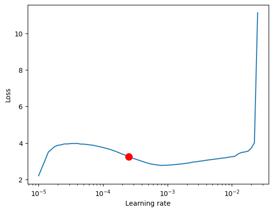
Finding the optimal learning rate using [PyTorch Lightning](https://pytorch-lightning.readthedocs.io/) is easy. The key hyperparameter of the NBeats model are the widths. Each denotes the width of each forecasting block. By default, the first forecasts the trend, while the second forecasts seasonality.

pl.seed_everything(42)
trainer = pl.Trainer(accelerator="auto", gradient_clip_val=0.01)
net = NBeats.from_dataset(training, learning_rate=3e-2, weight_decay=1e-2, widths=[32, 512], backcast_loss_ratio=0.1)

Global seed set to 42
GPU available: True (mps), used: True
TPU available: False, using: 0 TPU cores
IPU available: False, using: 0 IPUs
HPU available: False, using: 0 HPUs

# find optimal learning rate
from lightning.pytorch.tuner import Tuner

res = Tuner(trainer).lr_find(net, train_dataloaders=train_dataloader, val_dataloaders=val_dataloader, min_lr=1e-5)
print(f"suggested learning rate: {res.suggestion()}")
fig = res.plot(show=True, suggest=True)
fig.show()
net.hparams.learning_rate = res.suggestion()

LR finder stopped early after 68 steps due to diverging loss.
Learning rate set to 0.0002511886431509581
Restoring states from the checkpoint path at /Users/JanBeitner/Documents/code/pytorch-forecasting/.lr_find_6cdd9176-ee7a-4759-9728-172aaed215f7.ckpt
Restored all states from the checkpoint at /Users/JanBeitner/Documents/code/pytorch-forecasting/.lr_find_6cdd9176-ee7a-4759-9728-172aaed215f7.ckpt

suggested learning rate: 0.0002511886431509581

Fit model

early_stop_callback = EarlyStopping(monitor="val_loss", min_delta=1e-4, patience=10, verbose=False, mode="min")
trainer = pl.Trainer(
    max_epochs=3,
    accelerator="auto",
    enable_model_summary=True,
    gradient_clip_val=0.01,
    callbacks=[early_stop_callback],
    limit_train_batches=150,
)


net = NBeats.from_dataset(
    training,
    learning_rate=1e-3,
    log_interval=10,
    log_val_interval=1,
    weight_decay=1e-2,
    widths=[32, 512],
    backcast_loss_ratio=1.0,
)

trainer.fit(
    net,
    train_dataloaders=train_dataloader,
    val_dataloaders=val_dataloader,
)

GPU available: True (mps), used: True
TPU available: False, using: 0 TPU cores
IPU available: False, using: 0 IPUs
HPU available: False, using: 0 HPUs

  | Name            | Type       | Params
-----------------------------------------------
0 | loss            | MASE       | 0
1 | logging_metrics | ModuleList | 0
2 | net_blocks      | ModuleList | 1.7 M
-----------------------------------------------
1.7 M     Trainable params
0         Non-trainable params
1.7 M     Total params
6.851     Total estimated model params size (MB)

`Trainer.fit` stopped: `max_epochs=3` reached.

Evaluate Results

best_model_path = trainer.checkpoint_callback.best_model_path
best_model = NBeats.load_from_checkpoint(best_model_path)

We predict on the validation dataset with predict() and calculate the error which is well below the baseline error

actuals = torch.cat([y[0] for x, y in iter(val_dataloader)])
predictions = best_model.predict(val_dataloader)
(actuals - predictions).abs().mean()

tensor(0.1825)

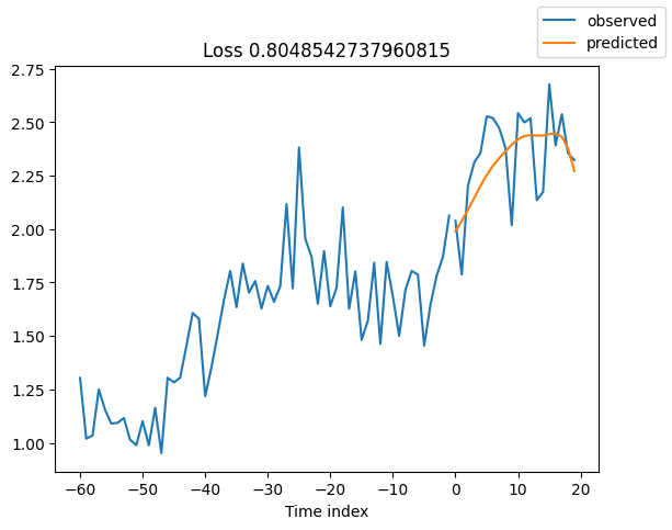
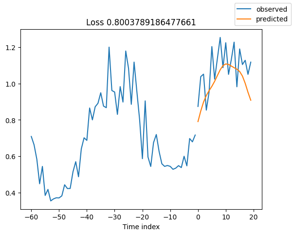
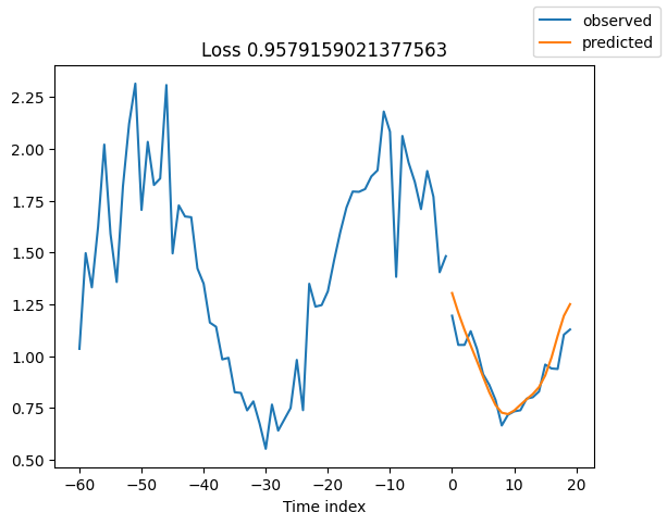
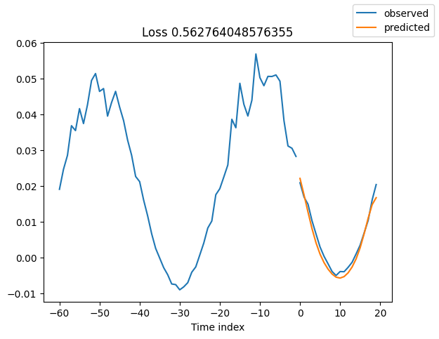
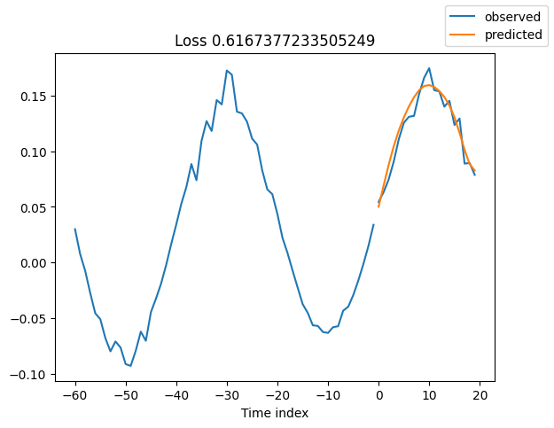
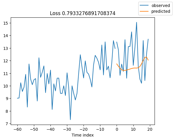
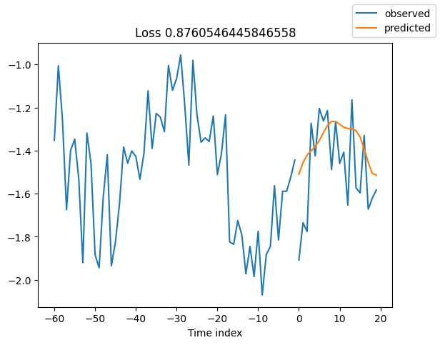
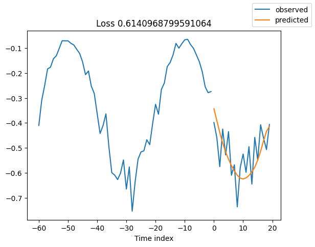
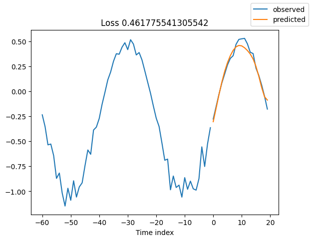
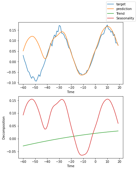
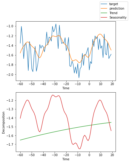
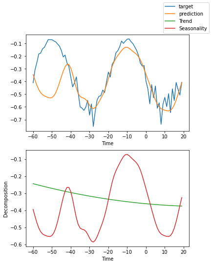
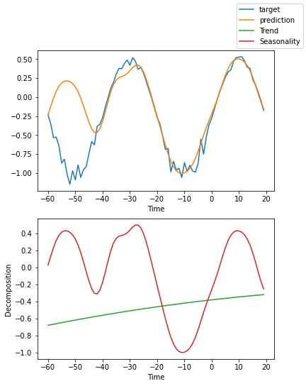
Looking at random samples from the validation set is always a good way to understand if the forecast is reasonable - and it is!

raw_predictions, x = best_model.predict(val_dataloader, mode="raw", return_x=True)

for idx in range(10):  # plot 10 examples
    best_model.plot_prediction(x, raw_predictions, idx=idx, add_loss_to_title=True)

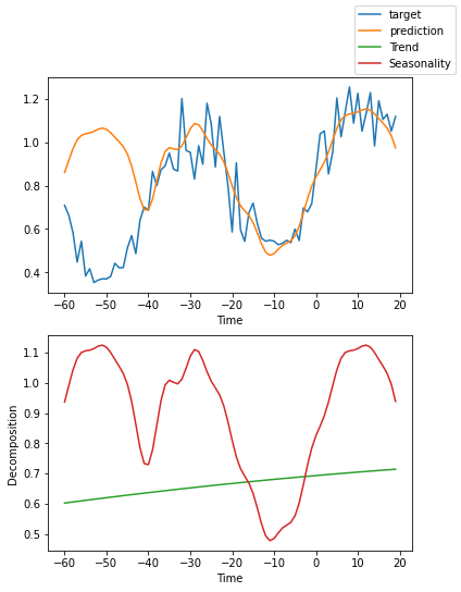
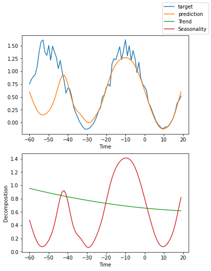
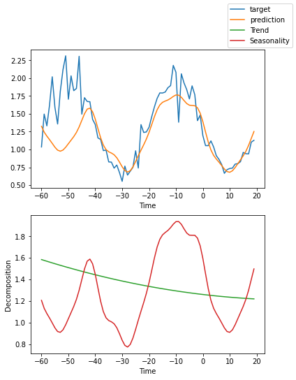
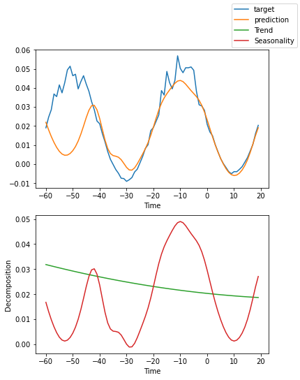
Interpret model

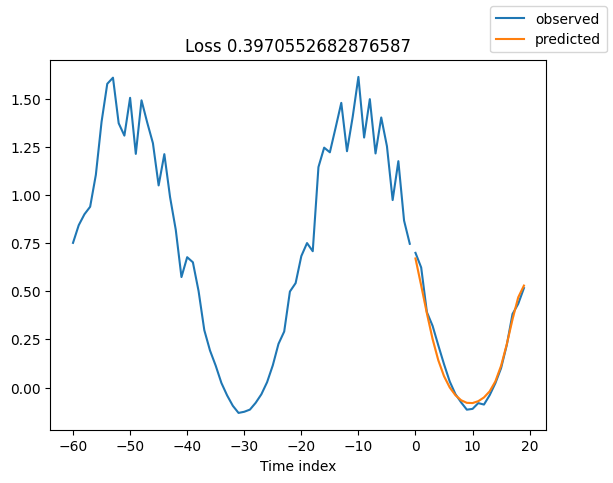
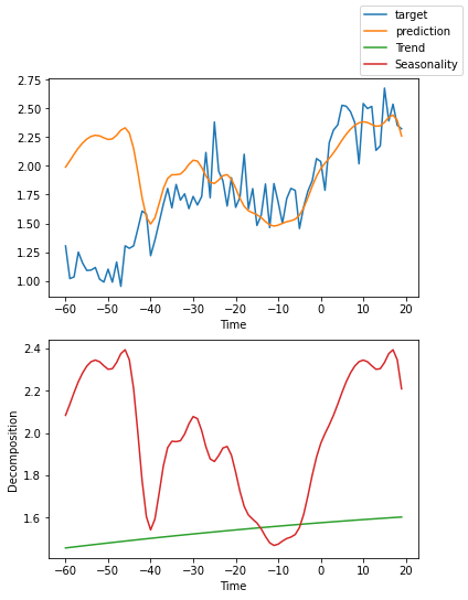
We can ask PyTorch Forecasting to decompose the prediction into seasonality and trend with plot_interpretation(). This is a special feature of the NBeats model and only possible because of its unique architecture. The results show that there seem to be many ways to explain the data and the algorithm does not always chooses the one making intuitive sense. This is partially down to the small number of time series we trained on (100). But it is also due because our forecasting period does not cover multiple seasonalities.

for idx in range(10):  # plot 10 examples
    best_model.plot_interpretation(x, raw_predictions, idx=idx)