Multivariate quantiles and long horizon forecasting with N-HiTS#
[1]:
import warnings

warnings.filterwarnings("ignore")
[2]:
import lightning.pytorch as pl
from lightning.pytorch.callbacks import EarlyStopping
import matplotlib.pyplot as plt
import numpy as np
import pandas as pd
import torch

from pytorch_forecasting import Baseline, NHiTS, TimeSeriesDataSet
from pytorch_forecasting.data import NaNLabelEncoder
from pytorch_forecasting.data.examples import generate_ar_data
from pytorch_forecasting.metrics import MAE, SMAPE, MQF2DistributionLoss, QuantileLoss
Load data#
We generate a synthetic dataset to demonstrate the network’s capabilities. The data consists of a quadratic trend and a seasonality component.
[3]:
data = generate_ar_data(seasonality=10.0, timesteps=400, n_series=100, seed=42)
data["static"] = 2
data["date"] = pd.Timestamp("2020-01-01") + pd.to_timedelta(data.time_idx, "D")
data.head()
[3]:
| series | time_idx | value | static | date | |
|---|---|---|---|---|---|
| 0 | 0 | 0 | -0.000000 | 2 | 2020-01-01 |
| 1 | 0 | 1 | -0.046501 | 2 | 2020-01-02 |
| 2 | 0 | 2 | -0.097796 | 2 | 2020-01-03 |
| 3 | 0 | 3 | -0.144397 | 2 | 2020-01-04 |
| 4 | 0 | 4 | -0.177954 | 2 | 2020-01-05 |
Before starting training, we need to split the dataset into a training and validation TimeSeriesDataSet.
[4]:
# create dataset and dataloaders
max_encoder_length = 60
max_prediction_length = 20

training_cutoff = data["time_idx"].max() - max_prediction_length

context_length = max_encoder_length
prediction_length = max_prediction_length

training = TimeSeriesDataSet(
    data[lambda x: x.time_idx <= training_cutoff],
    time_idx="time_idx",
    target="value",
    categorical_encoders={"series": NaNLabelEncoder().fit(data.series)},
    group_ids=["series"],
    # only unknown variable is "value" - and N-HiTS can also not take any additional variables
    time_varying_unknown_reals=["value"],
    max_encoder_length=context_length,
    max_prediction_length=prediction_length,
)

validation = TimeSeriesDataSet.from_dataset(
    training, data, min_prediction_idx=training_cutoff + 1
)
batch_size = 128
train_dataloader = training.to_dataloader(
    train=True, batch_size=batch_size, num_workers=0
)
val_dataloader = validation.to_dataloader(
    train=False, batch_size=batch_size, num_workers=0
)
Calculate baseline error#
Our baseline model predicts future values by repeating the last know value. The resulting SMAPE is disappointing and should not be easy to beat.
[5]:
# calculate baseline absolute error
baseline_predictions = Baseline().predict(
    val_dataloader, trainer_kwargs=dict(accelerator="cpu"), return_y=True
)
SMAPE()(baseline_predictions.output, baseline_predictions.y)
GPU available: True (mps), used: False
TPU available: False, using: 0 TPU cores
IPU available: False, using: 0 IPUs
HPU available: False, using: 0 HPUs
[5]:
tensor(0.5462)
Train network#
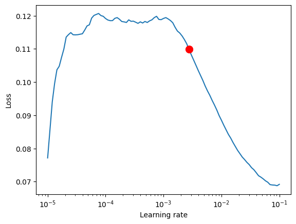
Finding the optimal learning rate using [PyTorch Lightning](https://pytorch-lightning.readthedocs.io/) is easy. The key hyperparameter of the NHiTS model is hidden_size.
PyTorch Forecasting is flexible enough to use NHiTS with different loss functions, enabling not only point forecasts but also probabilistic ones. Here, we will demonstrate not only a typical quantile regression but a multivariate quantile regression with MQF2DistributionLoss which allows calculation sampling consistent paths along a prediction horizon. This allows calculation of quantiles, e.g. of the sum over the prediction horizon while still avoiding the accumulating error problem from auto-regressive methods such as DeepAR. One needs to install an additional package for this quantile function:
pip install pytorch-forecasting[mqf2]
[6]:
pl.seed_everything(42)
trainer = pl.Trainer(accelerator="cpu", gradient_clip_val=0.1)
net = NHiTS.from_dataset(
    training,
    learning_rate=3e-2,
    weight_decay=1e-2,
    loss=MQF2DistributionLoss(prediction_length=max_prediction_length),
    backcast_loss_ratio=0.0,
    hidden_size=64,
    optimizer="AdamW",
)
Global seed set to 42
GPU available: True (mps), used: False
TPU available: False, using: 0 TPU cores
IPU available: False, using: 0 IPUs
HPU available: False, using: 0 HPUs
[ ]:
# find optimal learning rate
from pytorch_forecasting.tuning import Tuner

res = Tuner(trainer).lr_find(
    net,
    train_dataloaders=train_dataloader,
    val_dataloaders=val_dataloader,
    min_lr=1e-5,
    max_lr=1e-1,
)
print(f"suggested learning rate: {res.suggestion()}")
fig = res.plot(show=True, suggest=True)
net.hparams.learning_rate = res.suggestion()
`Trainer.fit` stopped: `max_steps=100` reached.
Learning rate set to 0.0027542287033381664
Restoring states from the checkpoint path at /Users/JanBeitner/Documents/code/pytorch-forecasting/.lr_find_9ea79aec-8577-4e17-859e-f46d818dbf70.ckpt
Restored all states from the checkpoint at /Users/JanBeitner/Documents/code/pytorch-forecasting/.lr_find_9ea79aec-8577-4e17-859e-f46d818dbf70.ckpt
suggested learning rate: 0.0027542287033381664
Fit model
[8]:
early_stop_callback = EarlyStopping(
    monitor="val_loss", min_delta=1e-4, patience=10, verbose=False, mode="min"
)
trainer = pl.Trainer(
    max_epochs=5,
    accelerator="cpu",
    enable_model_summary=True,
    gradient_clip_val=1.0,
    callbacks=[early_stop_callback],
    limit_train_batches=30,
    enable_checkpointing=True,
)


net = NHiTS.from_dataset(
    training,
    learning_rate=5e-3,
    log_interval=10,
    log_val_interval=1,
    weight_decay=1e-2,
    backcast_loss_ratio=0.0,
    hidden_size=64,
    optimizer="AdamW",
    loss=MQF2DistributionLoss(prediction_length=max_prediction_length),
)

trainer.fit(
    net,
    train_dataloaders=train_dataloader,
    val_dataloaders=val_dataloader,
)
GPU available: True (mps), used: False
TPU available: False, using: 0 TPU cores
IPU available: False, using: 0 IPUs
HPU available: False, using: 0 HPUs

  | Name            | Type                 | Params
---------------------------------------------------------
0 | loss            | MQF2DistributionLoss | 5.1 K
1 | logging_metrics | ModuleList           | 0
2 | embeddings      | MultiEmbedding       | 0
3 | model           | NHiTS                | 35.7 K
---------------------------------------------------------
40.8 K    Trainable params
0         Non-trainable params
40.8 K    Total params
0.163     Total estimated model params size (MB)
`Trainer.fit` stopped: `max_epochs=5` reached.
Evaluate Results#
[ ]:
best_model_path = trainer.checkpoint_callback.best_model_path
best_model = NHiTS.load_from_checkpoint(best_model_path)
We predict on the validation dataset with predict() and calculate the error which is well below the baseline error
[10]:
predictions = best_model.predict(
    val_dataloader, trainer_kwargs=dict(accelerator="cpu"), return_y=True
)
MAE()(predictions.output, predictions.y)
GPU available: True (mps), used: False
TPU available: False, using: 0 TPU cores
IPU available: False, using: 0 IPUs
HPU available: False, using: 0 HPUs
[10]:
tensor(0.2012)
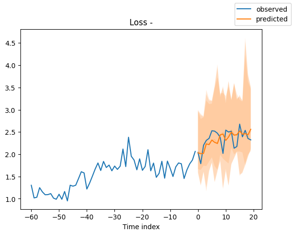
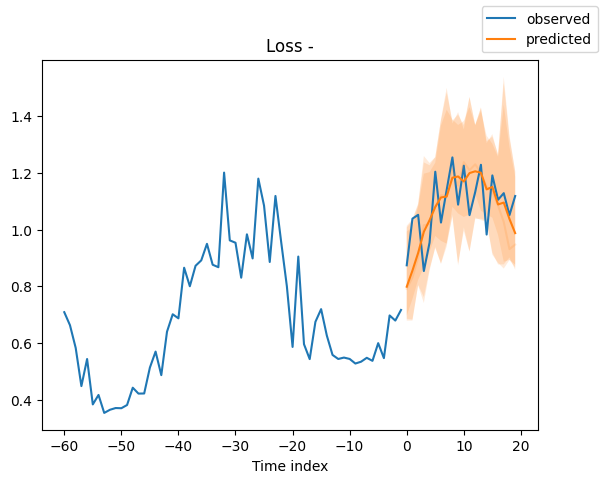
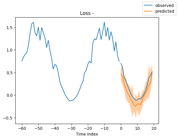
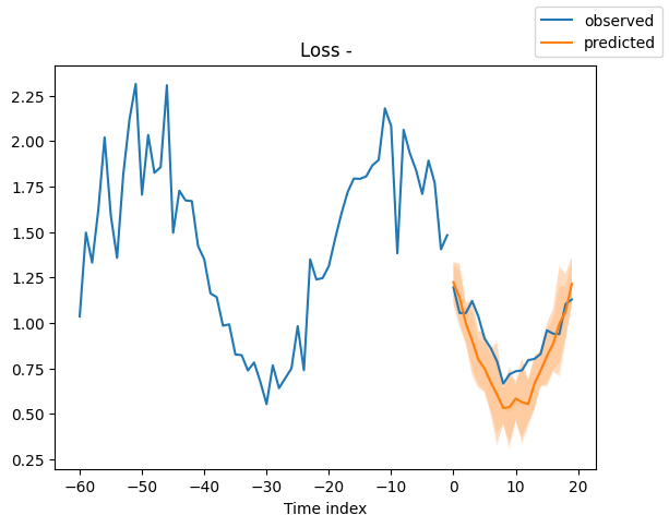
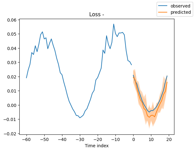
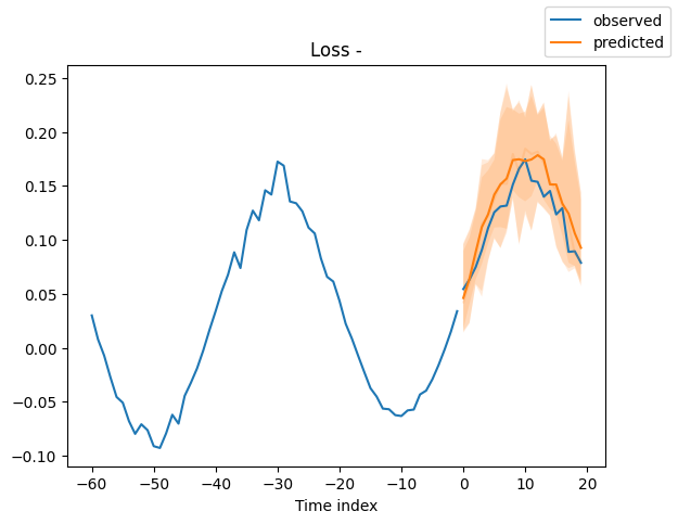
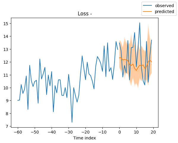
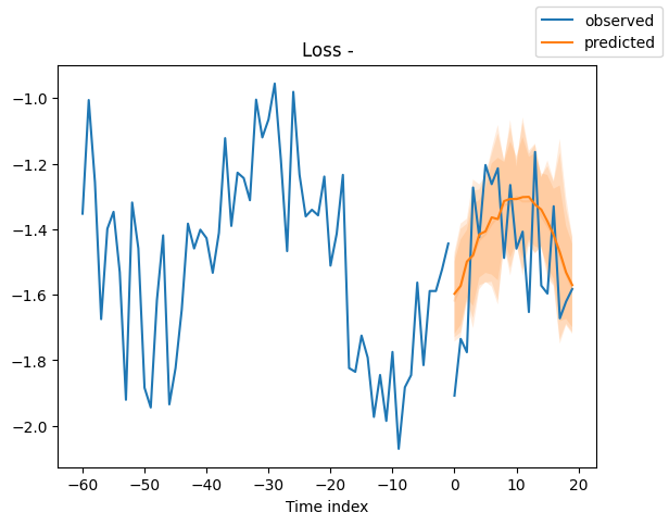
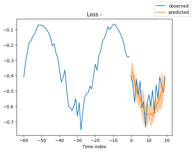
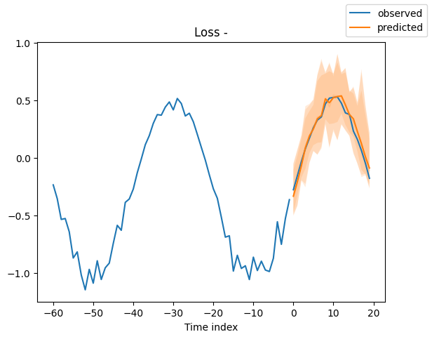
Looking at random samples from the validation set is always a good way to understand if the forecast is reasonable - and it is!
[11]:
raw_predictions = best_model.predict(
    val_dataloader, mode="raw", return_x=True, trainer_kwargs=dict(accelerator="cpu")
)
GPU available: True (mps), used: False
TPU available: False, using: 0 TPU cores
IPU available: False, using: 0 IPUs
HPU available: False, using: 0 HPUs
[12]:
for idx in range(10):  # plot 10 examples
    best_model.plot_prediction(
        raw_predictions.x, raw_predictions.output, idx=idx, add_loss_to_title=True
    )
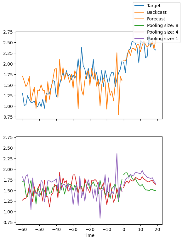
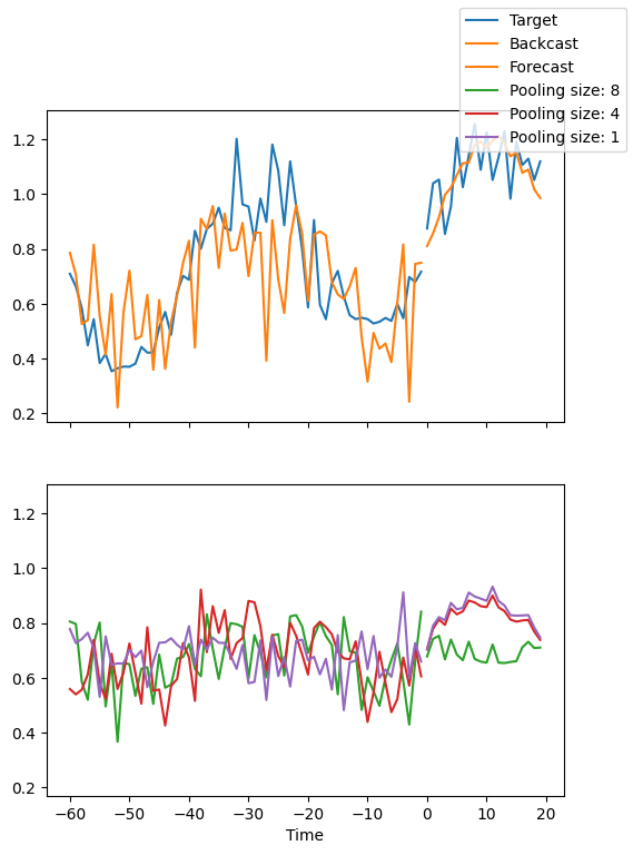
Interpret model#
We can ask PyTorch Forecasting to decompose the prediction into blocks which focus on a different frequency spectrum, e.g. seasonality and trend with plot_interpretation(). This is a special feature of the NHiTS model and only possible because of its unique architecture. The results show that there seem to be many ways to explain the data and the algorithm does not always chooses the one making intuitive sense. This is partially down to the small number of time series we trained on (100). But it is also due because our forecasting period does not cover multiple seasonalities.
[13]:
for idx in range(2):  # plot 10 examples
    best_model.plot_interpretation(raw_predictions.x, raw_predictions.output, idx=idx)
Sampling from predictions#
[14]:
# sample 500 paths
samples = best_model.loss.sample(
    raw_predictions.output["prediction"][[0]], n_samples=500
)[0]

# plot prediction
fig = best_model.plot_prediction(
    raw_predictions.x, raw_predictions.output, idx=0, add_loss_to_title=True
)
ax = fig.get_axes()[0]
# plot first two sampled paths
ax.plot(samples[:, 0], color="g", label="Sample 1")
ax.plot(samples[:, 1], color="r", label="Sample 2")
fig.legend()
[14]:
<matplotlib.legend.Legend at 0x2dea42680>
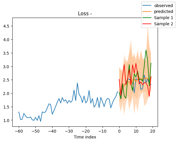
As expected, the variance of predictions is smaller within each sample than across all samples.
[15]:
print(f"Var(all samples) = {samples.var():.4f}")
print(f"Mean(Var(sample)) = {samples.var(0).mean():.4f}")
Var(all samples) = 0.2084
Mean(Var(sample)) = 0.1616
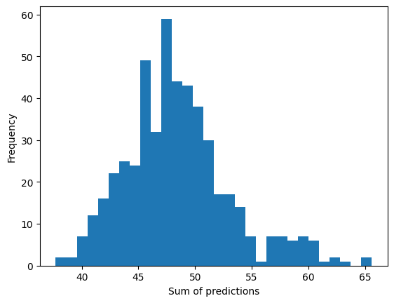
We can now do something new and plot the distribution of sums of forecasts over the entire prediction range.
[16]:
plt.hist(samples.sum(0).numpy(), bins=30)
plt.xlabel("Sum of predictions")
plt.ylabel("Frequency")
[16]:
Text(0, 0.5, 'Frequency')
[ ]:
[ ]: