Demand forecasting with the Temporal Fusion Transformer

In this tutorial, we will train the TemporalFusionTransformer on a very small dataset to demonstrate that it even does a good job on only 20k samples. Generally speaking, it is a large model and will therefore perform much better with more data.

Our example is a demand forecast from the Stallion kaggle competition.

import os
import warnings

warnings.filterwarnings("ignore")  # avoid printing out absolute paths

os.chdir("../../..")

import copy
from pathlib import Path
import warnings

import lightning.pytorch as pl
from lightning.pytorch.callbacks import EarlyStopping, LearningRateMonitor
from lightning.pytorch.loggers import TensorBoardLogger
import numpy as np
import pandas as pd
import torch

from pytorch_forecasting import Baseline, TemporalFusionTransformer, TimeSeriesDataSet
from pytorch_forecasting.data import GroupNormalizer
from pytorch_forecasting.metrics import MAE, SMAPE, PoissonLoss, QuantileLoss
from pytorch_forecasting.models.temporal_fusion_transformer.tuning import optimize_hyperparameters

Load data

First, we need to transform our time series into a pandas dataframe where each row can be identified with a time step and a time series. Fortunately, most datasets are already in this format. For this tutorial, we will use the Stallion dataset from Kaggle describing sales of various beverages. Our task is to make a six-month forecast of the sold volume by stock keeping units (SKU), that is products, sold by an agency, that is a store. There are about 21 000 monthly historic sales records. In addition to historic sales we have information about the sales price, the location of the agency, special days such as holidays, and volume sold in the entire industry.

The dataset is already in the correct format but misses some important features. Most importantly, we need to add a time index that is incremented by one for each time step. Further, it is beneficial to add date features, which in this case means extracting the month from the date record.

from pytorch_forecasting.data.examples import get_stallion_data

data = get_stallion_data()

# add time index
data["time_idx"] = data["date"].dt.year * 12 + data["date"].dt.month
data["time_idx"] -= data["time_idx"].min()

# add additional features
data["month"] = data.date.dt.month.astype(str).astype("category")  # categories have be strings
data["log_volume"] = np.log(data.volume + 1e-8)
data["avg_volume_by_sku"] = data.groupby(["time_idx", "sku"], observed=True).volume.transform("mean")
data["avg_volume_by_agency"] = data.groupby(["time_idx", "agency"], observed=True).volume.transform("mean")

# we want to encode special days as one variable and thus need to first reverse one-hot encoding
special_days = [
    "easter_day",
    "good_friday",
    "new_year",
    "christmas",
    "labor_day",
    "independence_day",
    "revolution_day_memorial",
    "regional_games",
    "fifa_u_17_world_cup",
    "football_gold_cup",
    "beer_capital",
    "music_fest",
]
data[special_days] = data[special_days].apply(lambda x: x.map({0: "-", 1: x.name})).astype("category")
data.sample(10, random_state=521)

	agency	sku	volume	date	industry_volume	soda_volume	avg_max_temp	price_regular	price_actual	discount	...	football_gold_cup	beer_capital	music_fest	discount_in_percent	timeseries	time_idx	month	log_volume	avg_volume_by_sku	avg_volume_by_agency
291	Agency_25	SKU_03	0.5076	2013-01-01	492612703	718394219	25.845238	1264.162234	1152.473405	111.688829	...	-	-	-	8.835008	228	0	1	-0.678062	1225.306376	99.650400
871	Agency_29	SKU_02	8.7480	2015-01-01	498567142	762225057	27.584615	1316.098485	1296.804924	19.293561	...	-	-	-	1.465966	177	24	1	2.168825	1634.434615	11.397086
19532	Agency_47	SKU_01	4.9680	2013-09-01	454252482	789624076	30.665957	1269.250000	1266.490490	2.759510	...	-	-	-	0.217413	322	8	9	1.603017	2625.472644	48.295650
2089	Agency_53	SKU_07	21.6825	2013-10-01	480693900	791658684	29.197727	1193.842373	1128.124395	65.717978	...	-	beer_capital	-	5.504745	240	9	10	3.076505	38.529107	2511.035175
9755	Agency_17	SKU_02	960.5520	2015-03-01	515468092	871204688	23.608120	1338.334248	1232.128069	106.206179	...	-	-	music_fest	7.935699	259	26	3	6.867508	2143.677462	396.022140
7561	Agency_05	SKU_03	1184.6535	2014-02-01	425528909	734443953	28.668254	1369.556376	1161.135214	208.421162	...	-	-	-	15.218151	21	13	2	7.077206	1566.643589	1881.866367
19204	Agency_11	SKU_05	5.5593	2017-08-01	623319783	1049868815	31.915385	1922.486644	1651.307674	271.178970	...	-	-	-	14.105636	17	55	8	1.715472	1385.225478	109.699200
8781	Agency_48	SKU_04	4275.1605	2013-03-01	509281531	892192092	26.767857	1761.258209	1546.059670	215.198539	...	-	-	music_fest	12.218455	151	2	3	8.360577	1757.950603	1925.272108
2540	Agency_07	SKU_21	0.0000	2015-10-01	544203593	761469815	28.987755	0.000000	0.000000	0.000000	...	-	-	-	0.000000	300	33	10	-18.420681	0.000000	2418.719550
12084	Agency_21	SKU_03	46.3608	2017-04-01	589969396	940912941	32.478910	1675.922116	1413.571789	262.350327	...	-	-	-	15.654088	181	51	4	3.836454	2034.293024	109.381800

10 rows × 31 columns

data.describe()

	volume	date	industry_volume	soda_volume	avg_max_temp	price_regular	price_actual	discount	avg_population_2017	avg_yearly_household_income_2017	discount_in_percent	timeseries	time_idx	log_volume	avg_volume_by_sku	avg_volume_by_agency
count	21000.000000	21000	2.100000e+04	2.100000e+04	21000.000000	21000.000000	21000.000000	21000.000000	2.100000e+04	21000.000000	21000.000000	21000.00000	21000.000000	21000.000000	21000.000000	21000.000000
mean	1492.403982	2015-06-16 20:48:00	5.439214e+08	8.512000e+08	28.612404	1451.536344	1267.347450	184.374146	1.045065e+06	151073.494286	10.574884	174.50000	29.500000	2.464118	1492.403982	1492.403982
min	0.000000	2013-01-01 00:00:00	4.130518e+08	6.964015e+08	16.731034	0.000000	-3121.690141	0.000000	1.227100e+04	90240.000000	0.000000	0.00000	0.000000	-18.420681	0.000000	0.000000
25%	8.272388	2014-03-24 06:00:00	5.090553e+08	7.890880e+08	25.374816	1311.547158	1178.365653	54.935108	6.018900e+04	110057.000000	3.749628	87.00000	14.750000	2.112923	932.285496	113.420250
50%	158.436000	2015-06-16 00:00:00	5.512000e+08	8.649196e+08	28.479272	1495.174592	1324.695705	138.307225	1.232242e+06	131411.000000	8.948990	174.50000	29.500000	5.065351	1402.305264	1730.529771
75%	1774.793475	2016-09-08 12:00:00	5.893715e+08	9.005551e+08	31.568405	1725.652080	1517.311427	272.298630	1.729177e+06	206553.000000	15.647058	262.00000	44.250000	7.481439	2195.362302	2595.316500
max	22526.610000	2017-12-01 00:00:00	6.700157e+08	1.049869e+09	45.290476	19166.625000	4925.404000	19166.625000	3.137874e+06	247220.000000	226.740147	349.00000	59.000000	10.022453	4332.363750	5884.717375
std	2711.496882	NaN	6.288022e+07	7.824340e+07	3.972833	683.362417	587.757323	257.469968	9.291926e+05	50409.593114	9.590813	101.03829	17.318515	8.178218	1051.790829	1328.239698

Create dataset and dataloaders

The next step is to convert the dataframe into a PyTorch Forecasting TimeSeriesDataSet. Apart from telling the dataset which features are categorical vs continuous and which are static vs varying in time, we also have to decide how we normalise the data. Here, we standard scale each time series separately and indicate that values are always positive. Generally, the EncoderNormalizer, that scales dynamically on each encoder sequence as you train, is preferred to avoid look-ahead bias induced by normalisation. However, you might accept look-ahead bias if you are having troubles to find a reasonably stable normalisation, for example, because there are a lot of zeros in your data. Or you expect a more stable normalization in inference. In the later case, you ensure that you do not learn “weird” jumps that will not be present when running inference, thus training on a more realistic data set.

We also choose to use the last six months as a validation set.

max_prediction_length = 6
max_encoder_length = 24
training_cutoff = data["time_idx"].max() - max_prediction_length

training = TimeSeriesDataSet(
    data[lambda x: x.time_idx <= training_cutoff],
    time_idx="time_idx",
    target="volume",
    group_ids=["agency", "sku"],
    min_encoder_length=max_encoder_length // 2,  # keep encoder length long (as it is in the validation set)
    max_encoder_length=max_encoder_length,
    min_prediction_length=1,
    max_prediction_length=max_prediction_length,
    static_categoricals=["agency", "sku"],
    static_reals=["avg_population_2017", "avg_yearly_household_income_2017"],
    time_varying_known_categoricals=["special_days", "month"],
    variable_groups={"special_days": special_days},  # group of categorical variables can be treated as one variable
    time_varying_known_reals=["time_idx", "price_regular", "discount_in_percent"],
    time_varying_unknown_categoricals=[],
    time_varying_unknown_reals=[
        "volume",
        "log_volume",
        "industry_volume",
        "soda_volume",
        "avg_max_temp",
        "avg_volume_by_agency",
        "avg_volume_by_sku",
    ],
    target_normalizer=GroupNormalizer(
        groups=["agency", "sku"], transformation="softplus"
    ),  # use softplus and normalize by group
    add_relative_time_idx=True,
    add_target_scales=True,
    add_encoder_length=True,
)

# create validation set (predict=True) which means to predict the last max_prediction_length points in time
# for each series
validation = TimeSeriesDataSet.from_dataset(training, data, predict=True, stop_randomization=True)

# create dataloaders for model
batch_size = 128  # set this between 32 to 128
train_dataloader = training.to_dataloader(train=True, batch_size=batch_size, num_workers=0)
val_dataloader = validation.to_dataloader(train=False, batch_size=batch_size * 10, num_workers=0)

To learn more about the TimeSeriesDataSet, visit its documentation or the tutorial explaining how to pass datasets to models.

Create baseline model

Evaluating a Baseline model that predicts the next 6 months by simply repeating the last observed volume gives us a simle benchmark that we want to outperform.

# calculate baseline mean absolute error, i.e. predict next value as the last available value from the history
baseline_predictions = Baseline().predict(val_dataloader, return_y=True)
MAE()(baseline_predictions.output, baseline_predictions.y)

tensor(293.0089, device='mps:0')

Train the Temporal Fusion Transformer

It is now time to create our TemporalFusionTransformer model. We train the model with PyTorch Lightning.

Find optimal learning rate

Prior to training, you can identify the optimal learning rate with the PyTorch Lightning learning rate finder.

# configure network and trainer
pl.seed_everything(42)
trainer = pl.Trainer(
    accelerator="cpu",
    # clipping gradients is a hyperparameter and important to prevent divergance
    # of the gradient for recurrent neural networks
    gradient_clip_val=0.1,
)


tft = TemporalFusionTransformer.from_dataset(
    training,
    # not meaningful for finding the learning rate but otherwise very important
    learning_rate=0.03,
    hidden_size=8,  # most important hyperparameter apart from learning rate
    # number of attention heads. Set to up to 4 for large datasets
    attention_head_size=1,
    dropout=0.1,  # between 0.1 and 0.3 are good values
    hidden_continuous_size=8,  # set to <= hidden_size
    loss=QuantileLoss(),
    optimizer="Ranger"
    # reduce learning rate if no improvement in validation loss after x epochs
    # reduce_on_plateau_patience=1000,
)
print(f"Number of parameters in network: {tft.size()/1e3:.1f}k")

Global seed set to 42
GPU available: True (mps), used: False
TPU available: False, using: 0 TPU cores
IPU available: False, using: 0 IPUs
HPU available: False, using: 0 HPUs

Number of parameters in network: 13.5k

# find optimal learning rate
from lightning.pytorch.tuner import Tuner

res = Tuner(trainer).lr_find(
    tft,
    train_dataloaders=train_dataloader,
    val_dataloaders=val_dataloader,
    max_lr=10.0,
    min_lr=1e-6,
)

print(f"suggested learning rate: {res.suggestion()}")
fig = res.plot(show=True, suggest=True)
fig.show()

`Trainer.fit` stopped: `max_steps=100` reached.
Learning rate set to 0.041686938347033554
Restoring states from the checkpoint path at /Users/JanBeitner/Documents/code/pytorch-forecasting/.lr_find_59af1c18-1ff9-46ba-b1b4-a6bcab492591.ckpt
Restored all states from the checkpoint at /Users/JanBeitner/Documents/code/pytorch-forecasting/.lr_find_59af1c18-1ff9-46ba-b1b4-a6bcab492591.ckpt

suggested learning rate: 0.041686938347033554

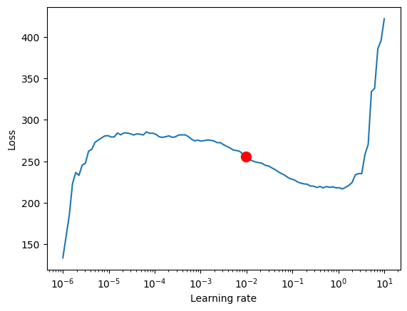
For the TemporalFusionTransformer, the optimal learning rate seems to be slightly lower than the suggested one. Further, we do not directly want to use the suggested learning rate because PyTorch Lightning sometimes can get confused by the noise at lower learning rates and suggests rates far too low. Manual control is essential. We decide to pick 0.03 as learning rate.

Train model

If you have troubles training the model and get an error AttributeError: module 'tensorflow._api.v2.io.gfile' has no attribute 'get_filesystem', consider either uninstalling tensorflow or first execute

import tensorflow as tf
import tensorboard as tb
tf.io.gfile = tb.compat.tensorflow_stub.io.gfile
```.

# configure network and trainer
early_stop_callback = EarlyStopping(monitor="val_loss", min_delta=1e-4, patience=10, verbose=False, mode="min")
lr_logger = LearningRateMonitor()  # log the learning rate
logger = TensorBoardLogger("lightning_logs")  # logging results to a tensorboard

trainer = pl.Trainer(
    max_epochs=50,
    accelerator="cpu",
    enable_model_summary=True,
    gradient_clip_val=0.1,
    limit_train_batches=50,  # coment in for training, running valiation every 30 batches
    # fast_dev_run=True,  # comment in to check that networkor dataset has no serious bugs
    callbacks=[lr_logger, early_stop_callback],
    logger=logger,
)

tft = TemporalFusionTransformer.from_dataset(
    training,
    learning_rate=0.03,
    hidden_size=16,
    attention_head_size=2,
    dropout=0.1,
    hidden_continuous_size=8,
    loss=QuantileLoss(),
    log_interval=10,  # uncomment for learning rate finder and otherwise, e.g. to 10 for logging every 10 batches
    optimizer="Ranger",
    reduce_on_plateau_patience=4,
)
print(f"Number of parameters in network: {tft.size()/1e3:.1f}k")

GPU available: True (mps), used: False
TPU available: False, using: 0 TPU cores
IPU available: False, using: 0 IPUs
HPU available: False, using: 0 HPUs

Number of parameters in network: 29.4k

Training takes a couple of minutes on my Macbook but for larger networks and datasets, it can take hours. The training speed is here mostly determined by overhead and choosing a larger batch_size or hidden_size (i.e. network size) does not slow does training linearly making training on large datasets feasible. During training, we can monitor the tensorboard which can be spun up with tensorboard --logdir=lightning_logs. For example, we can monitor examples predictions on the training and validation set.

# fit network
trainer.fit(
    tft,
    train_dataloaders=train_dataloader,
    val_dataloaders=val_dataloader,
)

   | Name                               | Type                            | Params
----------------------------------------------------------------------------------------
0  | loss                               | QuantileLoss                    | 0
1  | logging_metrics                    | ModuleList                      | 0
2  | input_embeddings                   | MultiEmbedding                  | 1.3 K
3  | prescalers                         | ModuleDict                      | 256
4  | static_variable_selection          | VariableSelectionNetwork        | 3.4 K
5  | encoder_variable_selection         | VariableSelectionNetwork        | 8.0 K
6  | decoder_variable_selection         | VariableSelectionNetwork        | 2.7 K
7  | static_context_variable_selection  | GatedResidualNetwork            | 1.1 K
8  | static_context_initial_hidden_lstm | GatedResidualNetwork            | 1.1 K
9  | static_context_initial_cell_lstm   | GatedResidualNetwork            | 1.1 K
10 | static_context_enrichment          | GatedResidualNetwork            | 1.1 K
11 | lstm_encoder                       | LSTM                            | 2.2 K
12 | lstm_decoder                       | LSTM                            | 2.2 K
13 | post_lstm_gate_encoder             | GatedLinearUnit                 | 544
14 | post_lstm_add_norm_encoder         | AddNorm                         | 32
15 | static_enrichment                  | GatedResidualNetwork            | 1.4 K
16 | multihead_attn                     | InterpretableMultiHeadAttention | 808
17 | post_attn_gate_norm                | GateAddNorm                     | 576
18 | pos_wise_ff                        | GatedResidualNetwork            | 1.1 K
19 | pre_output_gate_norm               | GateAddNorm                     | 576
20 | output_layer                       | Linear                          | 119
----------------------------------------------------------------------------------------
29.4 K    Trainable params
0         Non-trainable params
29.4 K    Total params
0.118     Total estimated model params size (MB)

Hyperparameter tuning

Hyperparamter tuning with [optuna](https://optuna.org/) is directly build into pytorch-forecasting. For example, we can use the optimize_hyperparameters() function to optimize the TFT’s hyperparameters.

import pickle

from pytorch_forecasting.models.temporal_fusion_transformer.tuning import optimize_hyperparameters

# create study
study = optimize_hyperparameters(
    train_dataloader,
    val_dataloader,
    model_path="optuna_test",
    n_trials=200,
    max_epochs=50,
    gradient_clip_val_range=(0.01, 1.0),
    hidden_size_range=(8, 128),
    hidden_continuous_size_range=(8, 128),
    attention_head_size_range=(1, 4),
    learning_rate_range=(0.001, 0.1),
    dropout_range=(0.1, 0.3),
    trainer_kwargs=dict(limit_train_batches=30),
    reduce_on_plateau_patience=4,
    use_learning_rate_finder=False,  # use Optuna to find ideal learning rate or use in-built learning rate finder
)

# save study results - also we can resume tuning at a later point in time
with open("test_study.pkl", "wb") as fout:
    pickle.dump(study, fout)

# show best hyperparameters
print(study.best_trial.params)

Evaluate performance

PyTorch Lightning automatically checkpoints training and thus, we can easily retrieve the best model and load it.

# load the best model according to the validation loss
# (given that we use early stopping, this is not necessarily the last epoch)
best_model_path = trainer.checkpoint_callback.best_model_path
best_tft = TemporalFusionTransformer.load_from_checkpoint(best_model_path)

After training, we can make predictions with predict(). The method allows very fine-grained control over what it returns so that, for example, you can easily match predictions to your pandas dataframe. See its documentation for details. We evaluate the metrics on the validation dataset and a couple of examples to see how well the model is doing. Given that we work with only 21 000 samples the results are very reassuring and can compete with results by a gradient booster. We also perform better than the baseline model. Given the noisy data, this is not trivial.

# calcualte mean absolute error on validation set
predictions = best_tft.predict(val_dataloader, return_y=True, trainer_kwargs=dict(accelerator="cpu"))
MAE()(predictions.output, predictions.y)

tensor(262.1610)

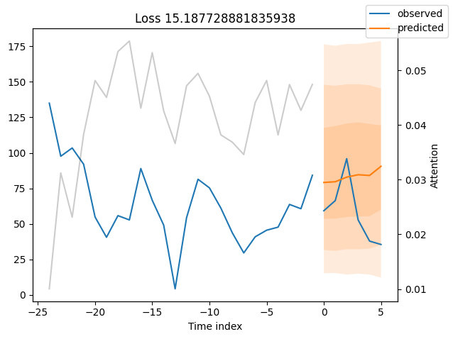
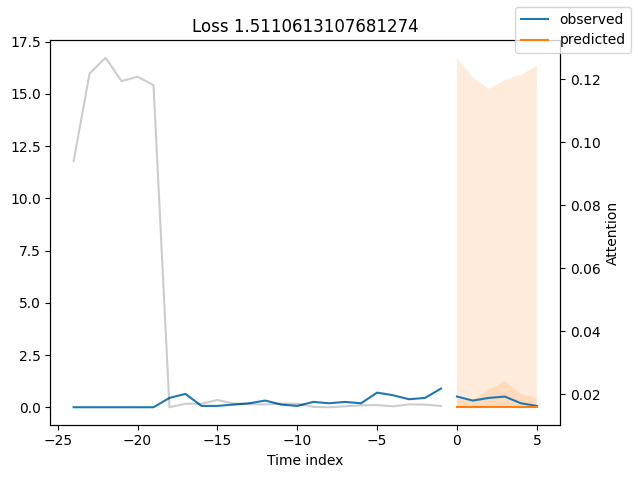
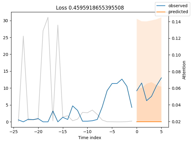
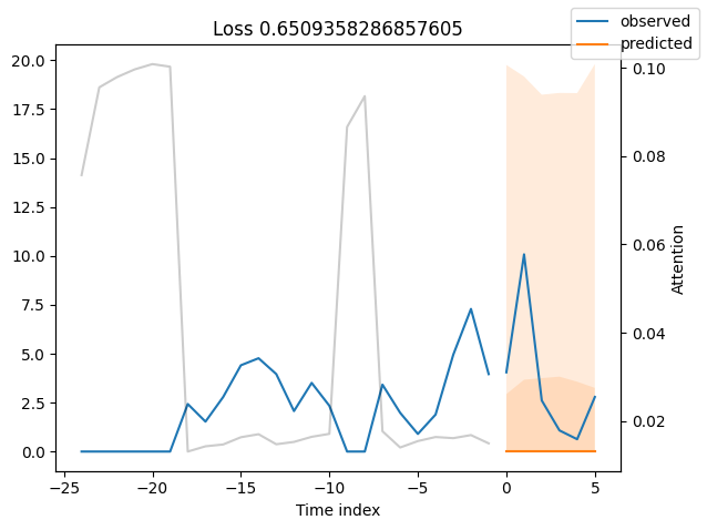
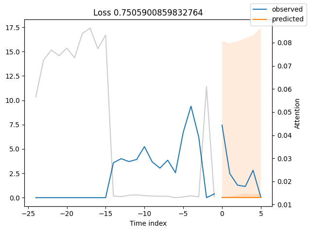
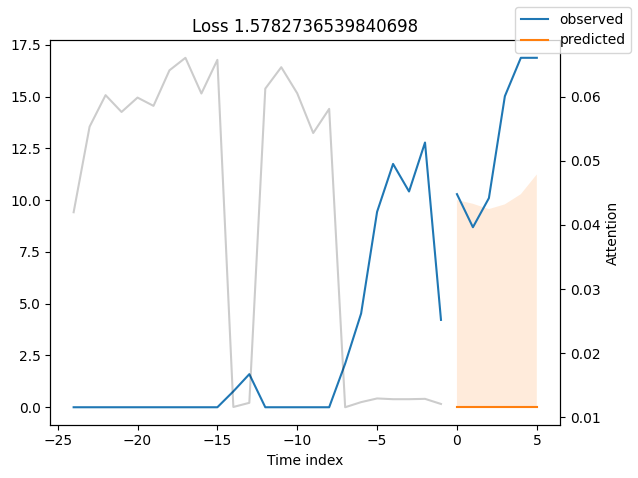
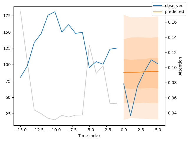
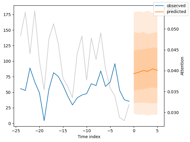
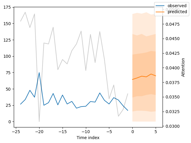
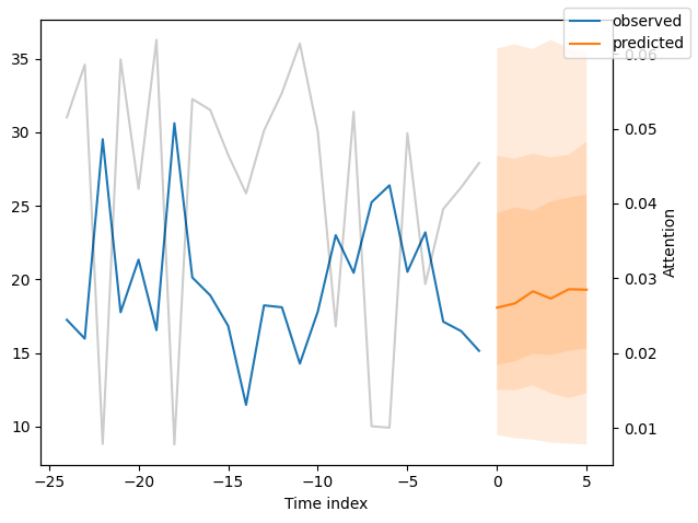
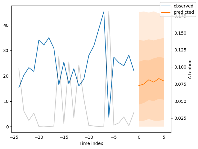
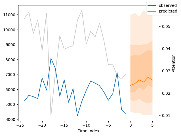
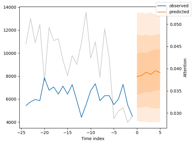
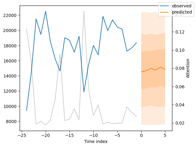
We can now also look at sample predictions directly which we plot with plot_prediction(). As you can see from the figures below, forecasts look rather accurate. If you wonder, the grey lines denote the amount of attention the model pays to different points in time when making the prediction. This is a special feature of the Temporal Fusion Transformer.

# raw predictions are a dictionary from which all kind of information including quantiles can be extracted
raw_predictions = best_tft.predict(val_dataloader, mode="raw", return_x=True)

for idx in range(10):  # plot 10 examples
    best_tft.plot_prediction(raw_predictions.x, raw_predictions.output, idx=idx, add_loss_to_title=True)

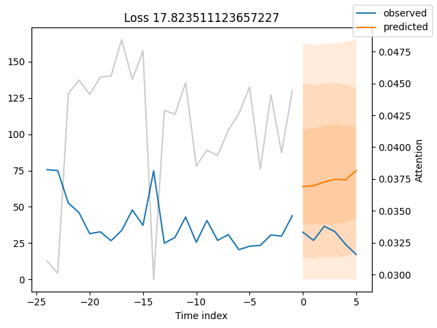
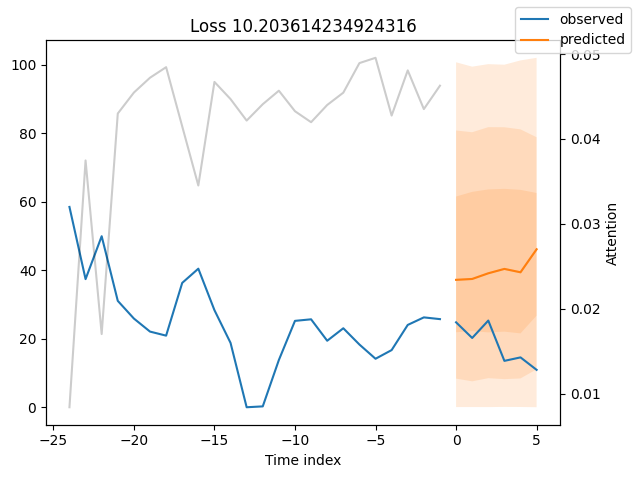
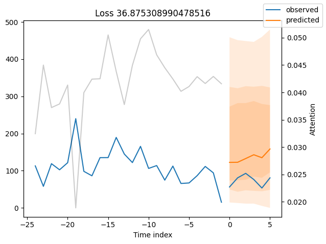
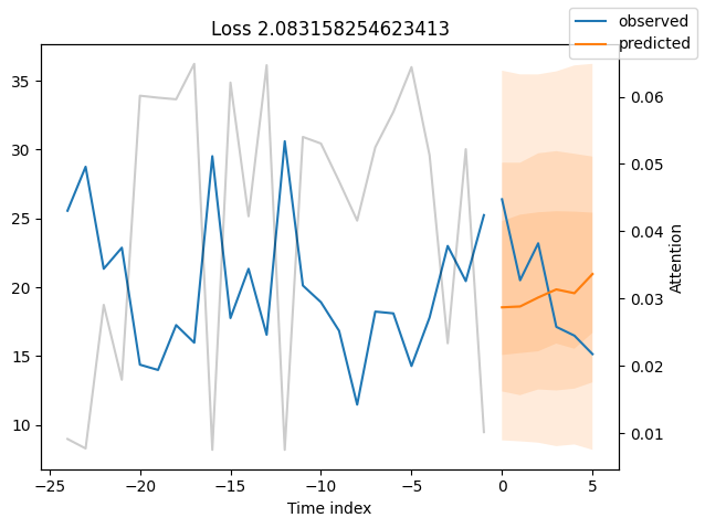
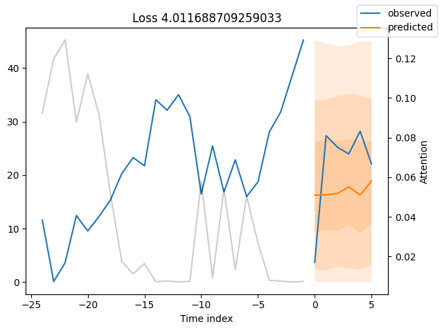
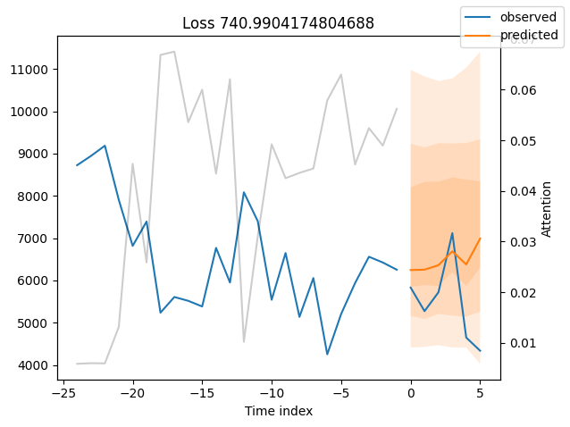
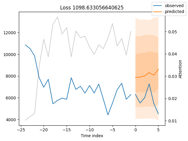
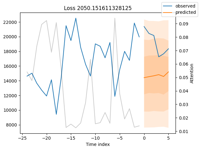
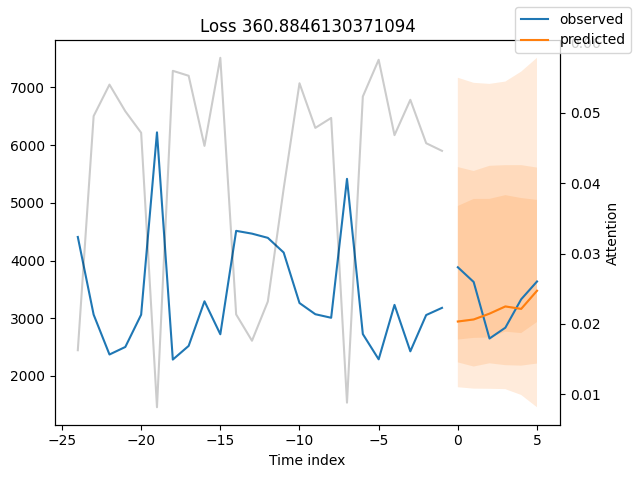
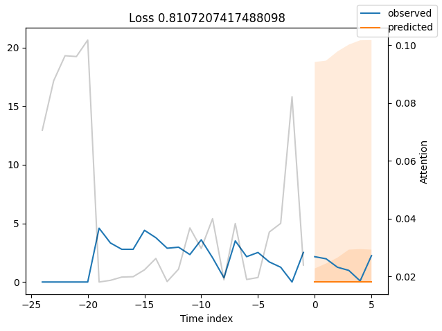
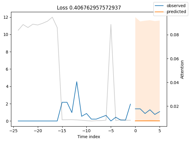
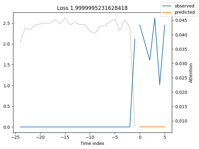
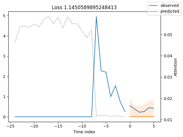
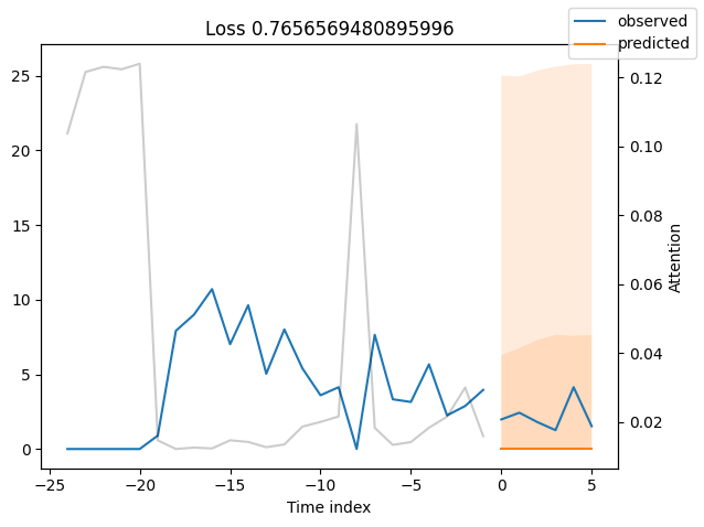
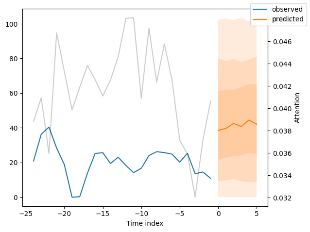
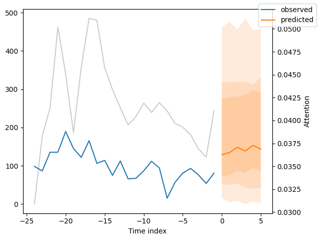
Worst performers

Looking at the worst performers, for example in terms of SMAPE, gives us an idea where the model has issues with forecasting reliably. These examples can provide important pointers about how to improve the model. This kind of actuals vs predictions plots are available to all models. Of course, it is also sensible to employ additional metrics, such as MASE, defined in the metrics module. However, for the sake of demonstration, we only use SMAPE here.

# calcualte metric by which to display
predictions = best_tft.predict(val_dataloader, return_y=True)
mean_losses = SMAPE(reduction="none")(predictions.output, predictions.y).mean(1)
indices = mean_losses.argsort(descending=True)  # sort losses
for idx in range(10):  # plot 10 examples
    best_tft.plot_prediction(
        raw_predictions.x,
        raw_predictions.output,
        idx=indices[idx],
        add_loss_to_title=SMAPE(quantiles=best_tft.loss.quantiles),
    )

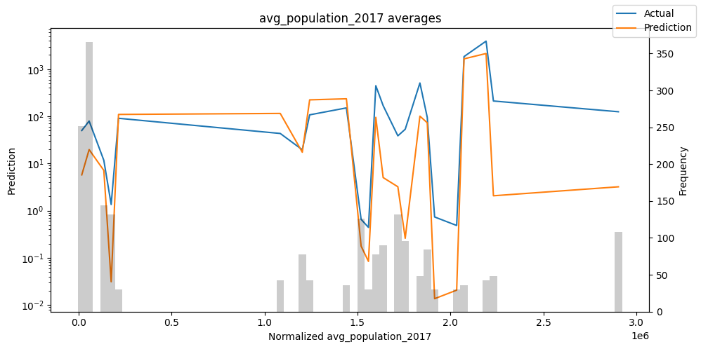
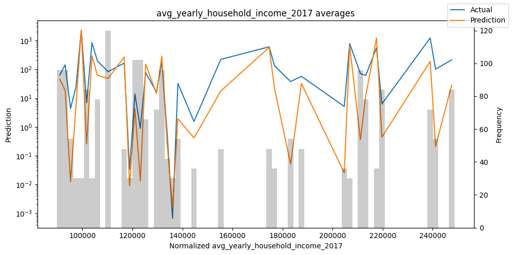
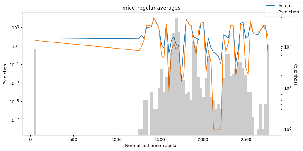
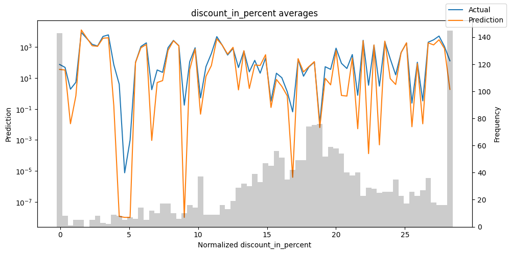
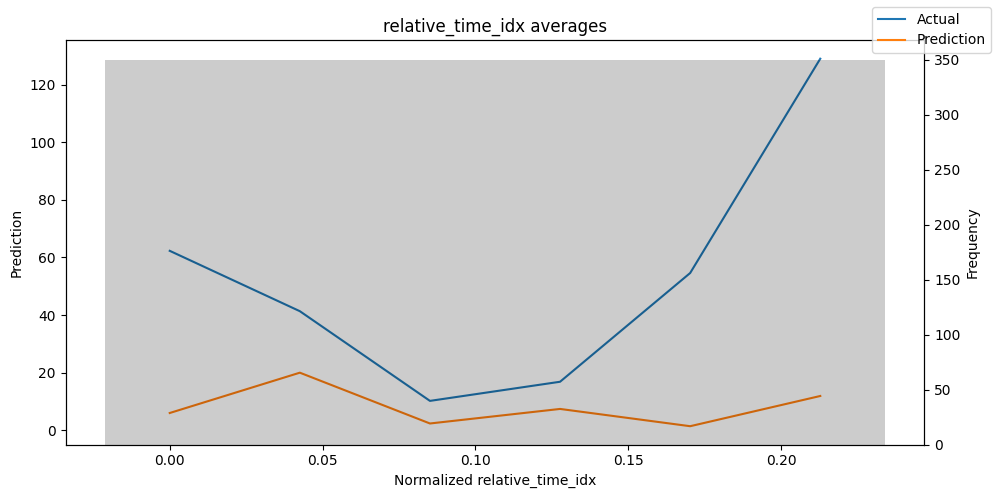
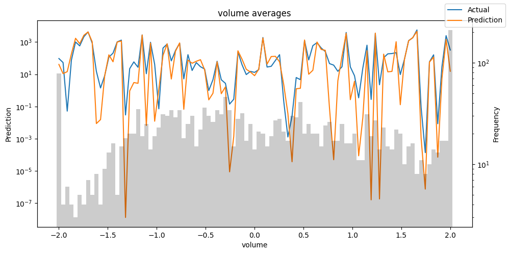
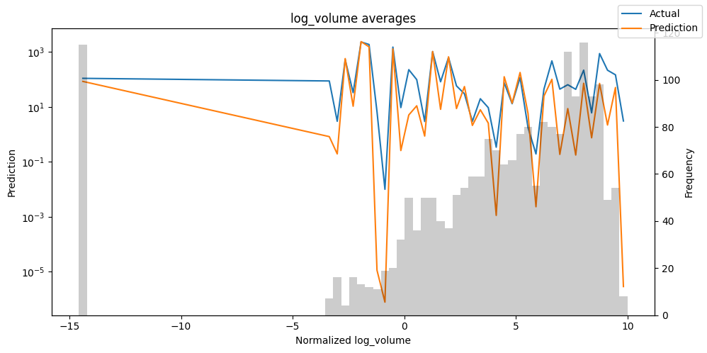
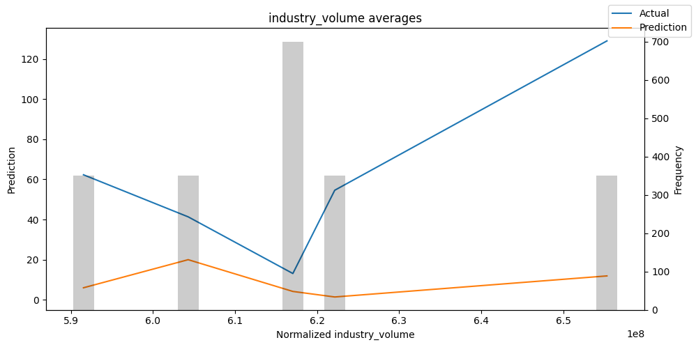
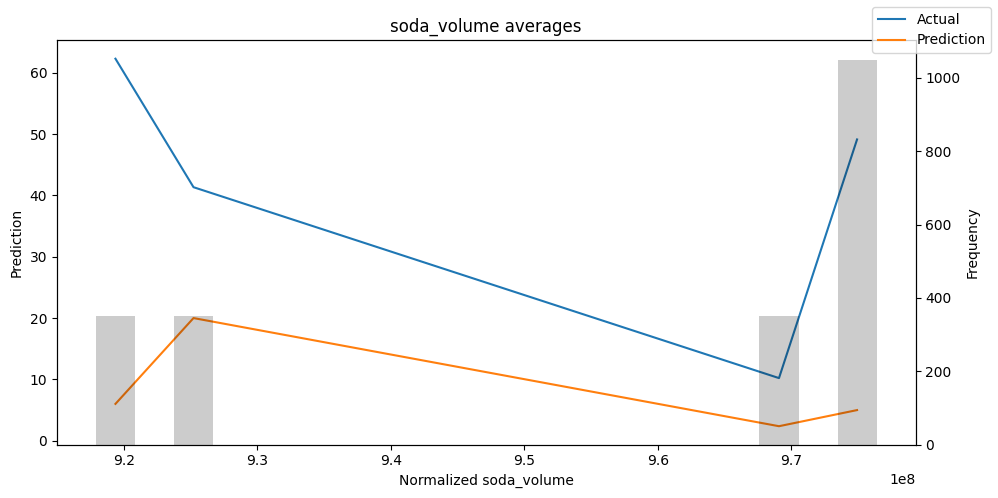
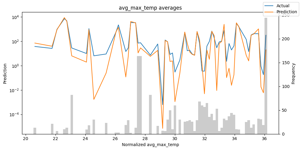
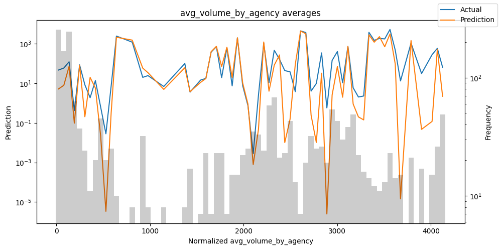
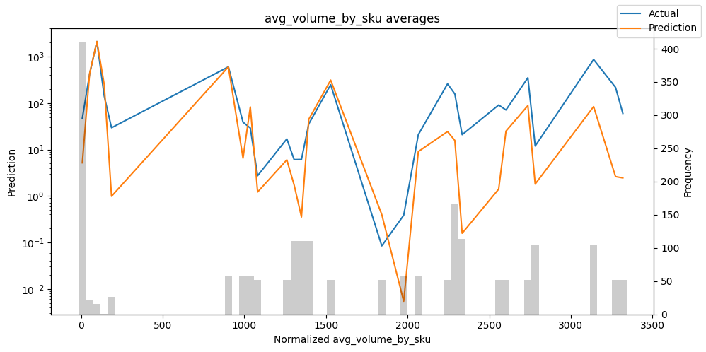
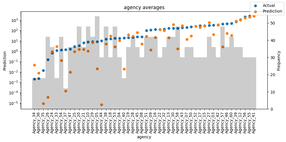
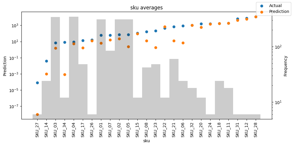
Actuals vs predictions by variables

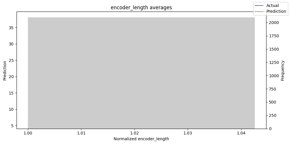
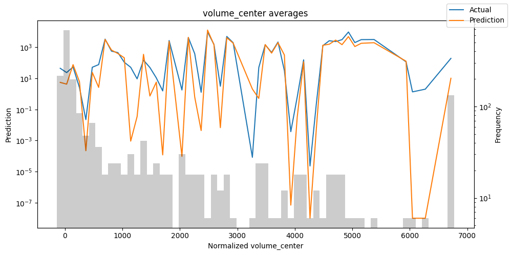
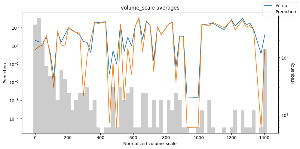
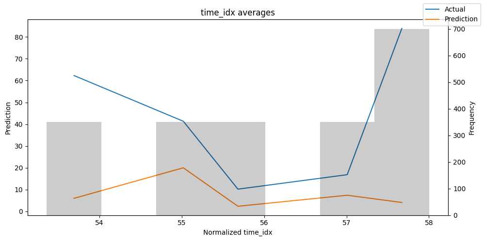
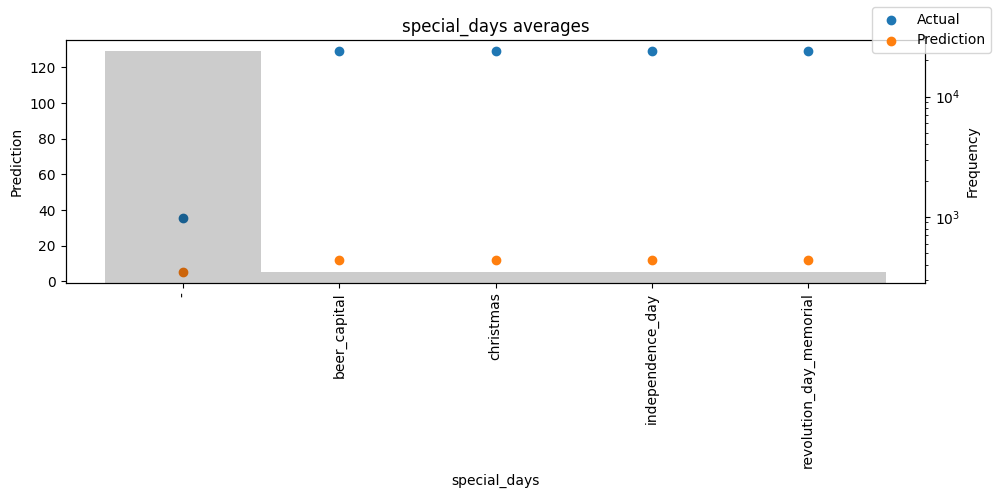
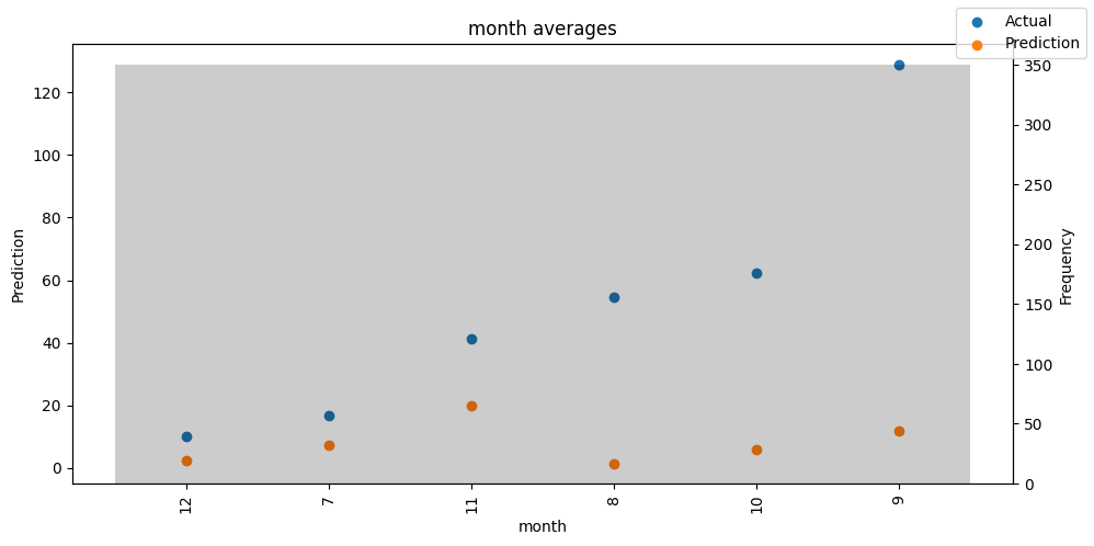
Checking how the model performs across different slices of the data allows us to detect weaknesses. Plotted below are the means of predictions vs actuals across each variable divided into 100 bins using the Now, we can directly predict on the generated data using the calculate_prediction_actual_by_variable() and plot_prediction_actual_by_variable() methods. The gray bars denote the frequency of the variable by bin, i.e. are a histogram.

predictions = best_tft.predict(val_dataloader, return_x=True)
predictions_vs_actuals = best_tft.calculate_prediction_actual_by_variable(predictions.x, predictions.output)
best_tft.plot_prediction_actual_by_variable(predictions_vs_actuals)

{'avg_population_2017': <Figure size 1000x500 with 2 Axes>,
 'avg_yearly_household_income_2017': <Figure size 1000x500 with 2 Axes>,
 'encoder_length': <Figure size 1000x500 with 2 Axes>,
 'volume_center': <Figure size 1000x500 with 2 Axes>,
 'volume_scale': <Figure size 1000x500 with 2 Axes>,
 'time_idx': <Figure size 1000x500 with 2 Axes>,
 'price_regular': <Figure size 1000x500 with 2 Axes>,
 'discount_in_percent': <Figure size 1000x500 with 2 Axes>,
 'relative_time_idx': <Figure size 1000x500 with 2 Axes>,
 'volume': <Figure size 1000x500 with 2 Axes>,
 'log_volume': <Figure size 1000x500 with 2 Axes>,
 'industry_volume': <Figure size 1000x500 with 2 Axes>,
 'soda_volume': <Figure size 1000x500 with 2 Axes>,
 'avg_max_temp': <Figure size 1000x500 with 2 Axes>,
 'avg_volume_by_agency': <Figure size 1000x500 with 2 Axes>,
 'avg_volume_by_sku': <Figure size 1000x500 with 2 Axes>,
 'agency': <Figure size 1000x500 with 2 Axes>,
 'sku': <Figure size 1000x500 with 2 Axes>,
 'special_days': <Figure size 1000x500 with 2 Axes>,
 'month': <Figure size 1000x500 with 2 Axes>}

Predict on selected data

To predict on a subset of data we can filter the subsequences in a dataset using the filter() method. Here we predict for the subsequence in the training dataset that maps to the group ids “Agency_01” and “SKU_01” and whose first predicted value corresponds to the time index “15”. We output all seven quantiles. This means we expect a tensor of shape 1 x n_timesteps x n_quantiles = 1 x 6 x 7 as we predict for a single subsequence six time steps ahead and 7 quantiles for each time step.

best_tft.predict(
    training.filter(lambda x: (x.agency == "Agency_01") & (x.sku == "SKU_01") & (x.time_idx_first_prediction == 15)),
    mode="quantiles",
)

tensor([[[ 71.8401,  95.7425, 110.2563, 130.6213, 147.2689, 164.7592, 183.4534],
         [ 26.5545,  56.0831,  73.5964,  98.4364, 117.8405, 141.8476, 163.2200],
         [ 19.5155,  46.8377,  62.4305,  86.6114, 104.1645, 126.8418, 147.6066],
         [ 34.3064,  58.6321,  72.5809,  93.5944, 110.5706, 129.0367, 154.7733],
         [ 28.2280,  53.3502,  67.4921,  88.0191, 104.0002, 120.7509, 141.0733],
         [ 17.6741,  42.3217,  55.3259,  77.8475,  93.1427, 112.8938, 135.0351]]],
       device='mps:0')

Of course, we can also plot this prediction readily:

raw_prediction = best_tft.predict(
    training.filter(lambda x: (x.agency == "Agency_01") & (x.sku == "SKU_01") & (x.time_idx_first_prediction == 15)),
    mode="raw",
    return_x=True,
)
best_tft.plot_prediction(raw_prediction.x, raw_prediction.output, idx=0)

Predict on new data

Because we have covariates in the dataset, predicting on new data requires us to define the known covariates upfront.

# select last 24 months from data (max_encoder_length is 24)
encoder_data = data[lambda x: x.time_idx > x.time_idx.max() - max_encoder_length]

# select last known data point and create decoder data from it by repeating it and incrementing the month
# in a real world dataset, we should not just forward fill the covariates but specify them to account
# for changes in special days and prices (which you absolutely should do but we are too lazy here)
last_data = data[lambda x: x.time_idx == x.time_idx.max()]
decoder_data = pd.concat(
    [last_data.assign(date=lambda x: x.date + pd.offsets.MonthBegin(i)) for i in range(1, max_prediction_length + 1)],
    ignore_index=True,
)

# add time index consistent with "data"
decoder_data["time_idx"] = decoder_data["date"].dt.year * 12 + decoder_data["date"].dt.month
decoder_data["time_idx"] += encoder_data["time_idx"].max() + 1 - decoder_data["time_idx"].min()

# adjust additional time feature(s)
decoder_data["month"] = decoder_data.date.dt.month.astype(str).astype("category")  # categories have be strings

# combine encoder and decoder data
new_prediction_data = pd.concat([encoder_data, decoder_data], ignore_index=True)

Now, we can directly predict on the generated data using the predict() method.

new_raw_predictions = best_tft.predict(new_prediction_data, mode="raw", return_x=True)

for idx in range(10):  # plot 10 examples
    best_tft.plot_prediction(new_raw_predictions.x, new_raw_predictions.output, idx=idx, show_future_observed=False)

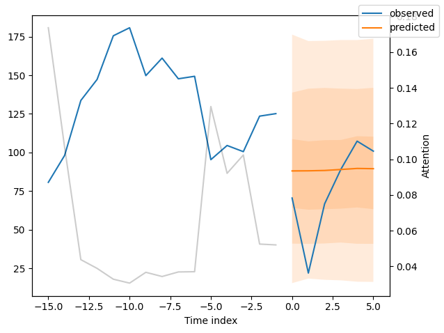
Interpret model

Variable importances

The model has inbuilt interpretation capabilities due to how its architecture is build. Let’s see how that looks. We first calculate interpretations with interpret_output() and plot them subsequently with plot_interpretation().

interpretation = best_tft.interpret_output(raw_predictions.output, reduction="sum")
best_tft.plot_interpretation(interpretation)

{'attention': <Figure size 640x480 with 1 Axes>,
 'static_variables': <Figure size 700x375 with 1 Axes>,
 'encoder_variables': <Figure size 700x525 with 1 Axes>,
 'decoder_variables': <Figure size 700x350 with 1 Axes>}

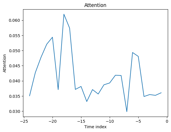
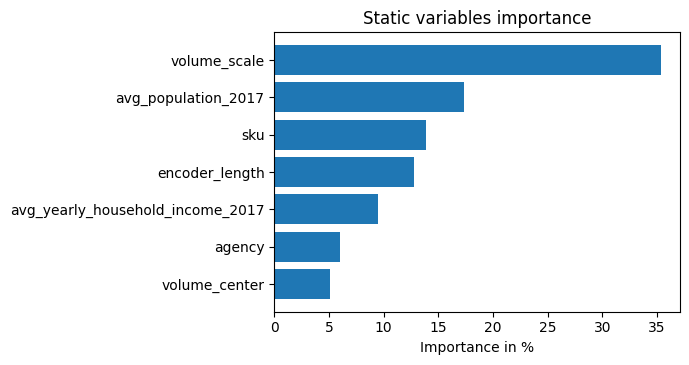
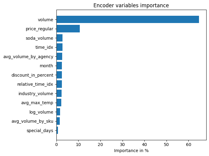
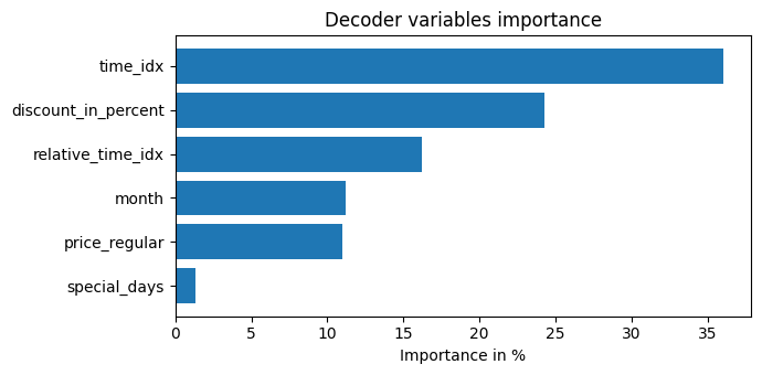
Unsurprisingly, the past observed volume features as the top variable in the encoder and price related variables are among the top predictors in the decoder.

The general attention patterns seems to be that more recent observations are more important and older ones. This confirms intuition. The average attention is often not very useful - looking at the attention by example is more insightful because patterns are not averaged out.

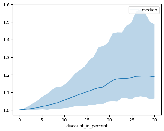
Partial dependency

Partial dependency plots are often used to interpret the model better (assuming independence of features). They can be also useful to understand what to expect in case of simulations and are created with predict_dependency().

dependency = best_tft.predict_dependency(
    val_dataloader.dataset, "discount_in_percent", np.linspace(0, 30, 30), show_progress_bar=True, mode="dataframe"
)

# plotting median and 25% and 75% percentile
agg_dependency = dependency.groupby("discount_in_percent").normalized_prediction.agg(
    median="median", q25=lambda x: x.quantile(0.25), q75=lambda x: x.quantile(0.75)
)
ax = agg_dependency.plot(y="median")
ax.fill_between(agg_dependency.index, agg_dependency.q25, agg_dependency.q75, alpha=0.3)

<matplotlib.collections.PolyCollection at 0x2db63e800>