How to use custom data and implement custom models and metrics

Building a new model in PyTorch Forecasting is relatively easy. Many things are taken care of automatically

• Training, validation and inference is automatically handled for most models - defining the architecture and hyperparameters is sufficient

• Dataloading, normalization, re-scaling etc. is provided by the TimeSeriesDataSet

• Logging training progress with multiple metrics including plotting examples is automatically taken care of

• Masking of entries if different time series have different lengths is automatic

However, there a couple of things to keep in mind if you want to make full use of the package. This tutorial first demonstrates how to implement a simple model and then turns to more complicated implementation scenarios.

We will answer questions such as

• How to transfer an existing PyTorch implementation into PyTorch Forecasting

• How to handle data loading and enable different length time series

• How to define and use a custom metric

• How to handle recurrent networks

• How to deal with covariates

• How to test new models

Building a simple, first model

For demonstration purposes we will choose a simple fully connected model. It takes a timeseries of size input_size as input and outputs a new timeseries of size output_size. You can think of this input_size encoding steps and output_size decoding/prediction steps.

import warnings

warnings.filterwarnings("ignore")

import torch
from torch import nn


class FullyConnectedModule(nn.Module):
    def __init__(self, input_size: int, output_size: int, hidden_size: int, n_hidden_layers: int):
        super().__init__()

        # input layer
        module_list = [nn.Linear(input_size, hidden_size), nn.ReLU()]
        # hidden layers
        for _ in range(n_hidden_layers):
            module_list.extend([nn.Linear(hidden_size, hidden_size), nn.ReLU()])
        # output layer
        module_list.append(nn.Linear(hidden_size, output_size))

        self.sequential = nn.Sequential(*module_list)

    def forward(self, x: torch.Tensor) -> torch.Tensor:
        # x of shape: batch_size x n_timesteps_in
        # output of shape batch_size x n_timesteps_out
        return self.sequential(x)


# test that network works as intended
network = FullyConnectedModule(input_size=5, output_size=2, hidden_size=10, n_hidden_layers=2)
x = torch.rand(20, 5)
network(x).shape

torch.Size([20, 2])

The above model is not yet a PyTorch Forecasting model but it is easy to get there. As this is a simple model, we will use the BaseModel. This base class is modified LightningModule with pre-defined hooks for training and validating time series models. The BaseModelWithCovariates will be discussed later in this tutorial.

Either way, the main requirement is for the model to have a forward method.

BaseModel.forward(x: Dict[str, List[Tensor] | Tensor]) → Dict[str, List[Tensor] | Tensor]

Network forward pass.

Parameters:

x (Dict[str, Union[torch.Tensor, List[torch.Tensor]]]) – network input (x as returned by the dataloader). See to_dataloader() method that returns a tuple of x and y. This function expects x.

Returns:

network outputs / dictionary of tensors or list

of tensors. Create it using the to_network_output() method. The minimal required entries in the dictionary are (and shapes in brackets):

• prediction (batch_size x n_decoder_time_steps x n_outputs or list thereof with each entry for a different target): re-scaled predictions that can be fed to metric. List of tensors if multiple targets are predicted at the same time.

Before passing outputting the predictions, you want to rescale them into real space. By default, you can use the transform_output() method to achieve this.

Return type:

NamedTuple[Union[torch.Tensor, List[torch.Tensor]]]

Example

def forward(self, x:
    # x is a batch generated based on the TimeSeriesDataset, here we just use the
    # continuous variables for the encoder
    network_input = x["encoder_cont"].squeeze(-1)
    prediction = self.linear(network_input)  #

    # rescale predictions into target space
    prediction = self.transform_output(prediction, target_scale=x["target_scale"])

    # We need to return a dictionary that at least contains the prediction
    # The parameter can be directly forwarded from the input.
    # The conversion to a named tuple can be directly achieved with the `to_network_output` function.
    return self.to_network_output(prediction=prediction)

from typing import Dict

from pytorch_forecasting.models import BaseModel


class FullyConnectedModel(BaseModel):
    def __init__(self, input_size: int, output_size: int, hidden_size: int, n_hidden_layers: int, **kwargs):
        # saves arguments in signature to `.hparams` attribute, mandatory call - do not skip this
        self.save_hyperparameters()
        # pass additional arguments to BaseModel.__init__, mandatory call - do not skip this
        super().__init__(**kwargs)
        self.network = FullyConnectedModule(
            input_size=self.hparams.input_size,
            output_size=self.hparams.output_size,
            hidden_size=self.hparams.hidden_size,
            n_hidden_layers=self.hparams.n_hidden_layers,
        )

    def forward(self, x: Dict[str, torch.Tensor]) -> Dict[str, torch.Tensor]:
        # x is a batch generated based on the TimeSeriesDataset
        network_input = x["encoder_cont"].squeeze(-1)
        prediction = self.network(network_input)

        # rescale predictions into target space
        prediction = self.transform_output(prediction, target_scale=x["target_scale"])

        # We need to return a dictionary that at least contains the prediction
        # The parameter can be directly forwarded from the input.
        # The conversion to a named tuple can be directly achieved with the `to_network_output` function.
        return self.to_network_output(prediction=prediction)

This is a very basic implementation that could be readily used for training. But before we add additional features, let’s first have a look how we pass data to this model before we go about initializing our model.

Passing data to a model

Instead of having to write our own dataloader (which can be rather complicated), we can leverage PyTorch Forecasting’s TimeSeriesDataSet to feed data to our model. In fact, PyTorch Forecasting expects us to use a TimeSeriesDataSet.

The data has to be in a specific format to be used by the TimeSeriesDataSet. It should be in a pandas DataFrame and have a categorical column to identify each series and a integer column to specify the time of the record.

Below, we create such a dataset with 30 different observations - 10 for 3 time series.

import numpy as np
import pandas as pd

test_data = pd.DataFrame(
    dict(
        value=np.random.rand(30) - 0.5,
        group=np.repeat(np.arange(3), 10),
        time_idx=np.tile(np.arange(10), 3),
    )
)
test_data

	value	group	time_idx
0	-0.125597	0	0
1	0.325668	0	1
2	-0.265962	0	2
3	0.132305	0	3
4	0.167117	0	4
5	0.481241	0	5
6	-0.113188	0	6
7	-0.089609	0	7
8	0.029156	0	8
9	-0.181950	0	9
10	0.150334	1	0
11	0.428624	1	1
12	-0.139106	1	2
13	-0.085334	1	3
14	-0.243668	1	4
15	0.055913	1	5
16	0.308591	1	6
17	0.141183	1	7
18	0.230759	1	8
19	0.173528	1	9
20	0.226315	2	0
21	-0.348390	2	1
22	0.067816	2	2
23	-0.074794	2	3
24	0.059396	2	4
25	0.300745	2	5
26	-0.344032	2	6
27	-0.083934	2	7
28	-0.343481	2	8
29	-0.385202	2	9

Converting it to a TimeSeriesDataSet is easy:

from pytorch_forecasting import TimeSeriesDataSet

# create the dataset from the pandas dataframe
dataset = TimeSeriesDataSet(
    test_data,
    group_ids=["group"],
    target="value",
    time_idx="time_idx",
    min_encoder_length=5,
    max_encoder_length=5,
    min_prediction_length=2,
    max_prediction_length=2,
    time_varying_unknown_reals=["value"],
)

We can take a look at all the defaults and settings that were set by PyTorch Forecasting. These are all available as arguments to TimeSeriesDataSet - see its documentation for more all the details.

dataset.get_parameters()

{'time_idx': 'time_idx',
 'target': 'value',
 'group_ids': ['group'],
 'weight': None,
 'max_encoder_length': 5,
 'min_encoder_length': 5,
 'min_prediction_idx': 0,
 'min_prediction_length': 2,
 'max_prediction_length': 2,
 'static_categoricals': [],
 'static_reals': [],
 'time_varying_known_categoricals': [],
 'time_varying_known_reals': [],
 'time_varying_unknown_categoricals': [],
 'time_varying_unknown_reals': ['value'],
 'variable_groups': {},
 'constant_fill_strategy': {},
 'allow_missing_timesteps': False,
 'lags': {},
 'add_relative_time_idx': False,
 'add_target_scales': False,
 'add_encoder_length': False,
 'target_normalizer': GroupNormalizer(
        method='standard',
        groups=[],
        center=True,
        scale_by_group=False,
        transformation=None,
        method_kwargs={}
 ),
 'categorical_encoders': {'__group_id__group': NaNLabelEncoder(add_nan=False, warn=True),
  'group': NaNLabelEncoder(add_nan=False, warn=True)},
 'scalers': {},
 'randomize_length': None,
 'predict_mode': False}

Now, we take a look at the output of the dataloader. It’s x will be fed to the model’s forward method, that is why it is so important to understand it.

# convert the dataset to a dataloader
dataloader = dataset.to_dataloader(batch_size=4)

# and load the first batch
x, y = next(iter(dataloader))
print("x =", x)
print("\ny =", y)
print("\nsizes of x =")
for key, value in x.items():
    print(f"\t{key} = {value.size()}")

x = {'encoder_cat': tensor([], size=(4, 5, 0), dtype=torch.int64), 'encoder_cont': tensor([[[ 1.7401],
         [-0.6492],
         [-0.4229],
         [-1.0892],
         [ 0.1716]],

        [[-0.4229],
         [-1.0892],
         [ 0.1716],
         [ 1.2349],
         [ 0.5304]],

        [[-0.6492],
         [-0.4229],
         [-1.0892],
         [ 0.1716],
         [ 1.2349]],

        [[-1.5299],
         [ 0.2216],
         [-0.3785],
         [ 0.1862],
         [ 1.2019]]]), 'encoder_target': tensor([[ 0.4286, -0.1391, -0.0853, -0.2437,  0.0559],
        [-0.0853, -0.2437,  0.0559,  0.3086,  0.1412],
        [-0.1391, -0.0853, -0.2437,  0.0559,  0.3086],
        [-0.3484,  0.0678, -0.0748,  0.0594,  0.3007]]), 'encoder_lengths': tensor([5, 5, 5, 5]), 'decoder_cat': tensor([], size=(4, 2, 0), dtype=torch.int64), 'decoder_cont': tensor([[[ 1.2349],
         [ 0.5304]],

        [[ 0.9074],
         [ 0.6665]],

        [[ 0.5304],
         [ 0.9074]],

        [[-1.5116],
         [-0.4170]]]), 'decoder_target': tensor([[ 0.3086,  0.1412],
        [ 0.2308,  0.1735],
        [ 0.1412,  0.2308],
        [-0.3440, -0.0839]]), 'decoder_lengths': tensor([2, 2, 2, 2]), 'decoder_time_idx': tensor([[6, 7],
        [8, 9],
        [7, 8],
        [6, 7]]), 'groups': tensor([[1],
        [1],
        [1],
        [2]]), 'target_scale': tensor([[0.0151, 0.2376],
        [0.0151, 0.2376],
        [0.0151, 0.2376],
        [0.0151, 0.2376]])}

y = (tensor([[ 0.3086,  0.1412],
        [ 0.2308,  0.1735],
        [ 0.1412,  0.2308],
        [-0.3440, -0.0839]]), None)

sizes of x =
        encoder_cat = torch.Size([4, 5, 0])
        encoder_cont = torch.Size([4, 5, 1])
        encoder_target = torch.Size([4, 5])
        encoder_lengths = torch.Size([4])
        decoder_cat = torch.Size([4, 2, 0])
        decoder_cont = torch.Size([4, 2, 1])
        decoder_target = torch.Size([4, 2])
        decoder_lengths = torch.Size([4])
        decoder_time_idx = torch.Size([4, 2])
        groups = torch.Size([4, 1])
        target_scale = torch.Size([4, 2])

To understand it better, we look at documentation of the to_dataloader() method:

TimeSeriesDataSet.to_dataloader(train: bool = True, batch_size: int = 64, batch_sampler: Sampler | str = None, **kwargs) → DataLoader

Get dataloader from dataset.

The

Parameters:

• train (bool, optional) – if dataloader is used for training or prediction Will shuffle and drop last batch if True. Defaults to True.

• batch_size (int) – batch size for training model. Defaults to 64.

• batch_sampler (Union[Sampler, str]) –

  batch sampler or string. One of

  • ”synchronized”: ensure that samples in decoder are aligned in time. Does not support missing values in dataset. This makes only sense if the underlying algorithm makes use of values aligned in time.

  • PyTorch Sampler instance: any PyTorch sampler, e.g. the WeightedRandomSampler()

  • None: samples are taken randomly from times series.

• **kwargs – additional arguments to DataLoader()

Returns:

dataloader that returns Tuple.

First entry is x, a dictionary of tensors with the entries (and shapes in brackets)

• encoder_cat (batch_size x n_encoder_time_steps x n_features): long tensor of encoded categoricals for encoder

• encoder_cont (batch_size x n_encoder_time_steps x n_features): float tensor of scaled continuous variables for encoder

• encoder_target (batch_size x n_encoder_time_steps or list thereof with each entry for a different target): float tensor with unscaled continous target or encoded categorical target, list of tensors for multiple targets

• encoder_lengths (batch_size): long tensor with lengths of the encoder time series. No entry will be greater than n_encoder_time_steps

• decoder_cat (batch_size x n_decoder_time_steps x n_features): long tensor of encoded categoricals for decoder

• decoder_cont (batch_size x n_decoder_time_steps x n_features): float tensor of scaled continuous variables for decoder

• decoder_target (batch_size x n_decoder_time_steps or list thereof with each entry for a different target): float tensor with unscaled continous target or encoded categorical target for decoder - this corresponds to first entry of y, list of tensors for multiple targets

• decoder_lengths (batch_size): long tensor with lengths of the decoder time series. No entry will be greater than n_decoder_time_steps

• group_ids (batch_size x number_of_ids): encoded group ids that identify a time series in the dataset

• target_scale (batch_size x scale_size or list thereof with each entry for a different target): parameters used to normalize the target. Typically these are mean and standard deviation. Is list of tensors for multiple targets.

Second entry is y, a tuple of the form (target, weight)

• target (batch_size x n_decoder_time_steps or list thereof with each entry for a different target): unscaled (continuous) or encoded (categories) targets, list of tensors for multiple targets

• weight (None or batch_size x n_decoder_time_steps): weight

Return type:

DataLoader

Example

Weight by samples for training:

from torch.utils.data import WeightedRandomSampler

# length of probabilties for sampler have to be equal to the length of the index
probabilities = np.sqrt(1 + data.loc[dataset.index, "target"])
sampler = WeightedRandomSampler(probabilities, len(probabilities))
dataset.to_dataloader(train=True, sampler=sampler, shuffle=False)

This explains why we had to first extract the correct input in our simple FullyConnectedModel above before passing it to our FullyConnectedModule. As a reminder:

def forward(self, x: Dict[str, torch.Tensor]) -> Dict[str, torch.Tensor]:
    # x is a batch generated based on the TimeSeriesDataset
    network_input = x["encoder_cont"].squeeze(-1)
    prediction = self.network(network_input)

    # rescale predictions into target space
    prediction = self.transform_output(prediction, target_scale=x["target_scale"])

    # We need to return a dictionary that at least contains the prediction
    # The parameter can be directly forwarded from the input.
    # The conversion to a named tuple can be directly achieved with the `to_network_output` function.
    return self.to_network_output(prediction=prediction)

For such a simple architecture, we can ignore most of the inputs in x. You do not have to worry about moving tensors to specifc GPUs, PyTorch Lightning will take care of this for you.

Now, let’s check if our model works. We initialize model always with their from_dataset() method with takes hyperparameters from the dataset, hyperparameters for the model and hyperparameters for the optimizer. Read more about it in the next section.

model = FullyConnectedModel.from_dataset(dataset, input_size=5, output_size=2, hidden_size=10, n_hidden_layers=2)
x, y = next(iter(dataloader))
model(x)

Output(prediction=tensor([[-0.0175, -0.0045],
        [-0.0203,  0.0039],
        [-0.0128,  0.0033],
        [-0.0162, -0.0026]], grad_fn=<AddBackward0>))

If you want to know to which group and time index (at the first prediction) the samples in the batch link to, you can find out by using x_to_index():

dataset.x_to_index(x)

	time_idx	group
0	5	2
1	5	1
2	7	2
3	5	0

Coupling datasets and models

You might have noticed that the encoder and decoder/prediction lengths (5 and 2) are already specified in the TimeSeriesDataSet and we specified them a second time when initializing the model. This might be acceptable for such a simple model but will make it hard for users to understand how to map form the dataset to the model parameters in more complicated settings. This is why we should implement another method in the model: from_dataset(). Typically, a user would always initialize a model from a dataset. The method is also an opportunity to validate that the dataset defined by the user is compatible with your model architecture.

While the TimeSeriesDataSet and all PyTorch Forecasting metrics support different length time series, not every network architecture does.

class FullyConnectedModel(BaseModel):
    def __init__(self, input_size: int, output_size: int, hidden_size: int, n_hidden_layers: int, **kwargs):
        # saves arguments in signature to `.hparams` attribute, mandatory call - do not skip this
        self.save_hyperparameters()
        # pass additional arguments to BaseModel.__init__, mandatory call - do not skip this
        super().__init__(**kwargs)
        self.network = FullyConnectedModule(
            input_size=self.hparams.input_size,
            output_size=self.hparams.output_size,
            hidden_size=self.hparams.hidden_size,
            n_hidden_layers=self.hparams.n_hidden_layers,
        )

    def forward(self, x: Dict[str, torch.Tensor]) -> Dict[str, torch.Tensor]:
        # x is a batch generated based on the TimeSeriesDataset
        network_input = x["encoder_cont"].squeeze(-1)
        prediction = self.network(network_input).unsqueeze(-1)

        # rescale predictions into target space
        prediction = self.transform_output(prediction, target_scale=x["target_scale"])

        # We need to return a dictionary that at least contains the prediction.
        # The parameter can be directly forwarded from the input.
        # The conversion to a named tuple can be directly achieved with the `to_network_output` function.
        return self.to_network_output(prediction=prediction)

    @classmethod
    def from_dataset(cls, dataset: TimeSeriesDataSet, **kwargs):
        new_kwargs = {
            "output_size": dataset.max_prediction_length,
            "input_size": dataset.max_encoder_length,
        }
        new_kwargs.update(kwargs)  # use to pass real hyperparameters and override defaults set by dataset
        # example for dataset validation
        assert dataset.max_prediction_length == dataset.min_prediction_length, "Decoder only supports a fixed length"
        assert dataset.min_encoder_length == dataset.max_encoder_length, "Encoder only supports a fixed length"
        assert (
            len(dataset._time_varying_known_categoricals) == 0
            and len(dataset._time_varying_known_reals) == 0
            and len(dataset._time_varying_unknown_categoricals) == 0
            and len(dataset._static_categoricals) == 0
            and len(dataset._static_reals) == 0
            and len(dataset._time_varying_unknown_reals) == 1
            and dataset._time_varying_unknown_reals[0] == dataset.target
        ), "Only covariate should be the target in 'time_varying_unknown_reals'"

        return super().from_dataset(dataset, **new_kwargs)

Now, let’s initialize from our dataset:

from lightning.pytorch.utilities.model_summary import ModelSummary

model = FullyConnectedModel.from_dataset(dataset, hidden_size=10, n_hidden_layers=2)
print(ModelSummary(model, max_depth=-1))
model.hparams

   | Name                 | Type                 | Params
---------------------------------------------------------------
0  | loss                 | SMAPE                | 0
1  | logging_metrics      | ModuleList           | 0
2  | network              | FullyConnectedModule | 302
3  | network.sequential   | Sequential           | 302
4  | network.sequential.0 | Linear               | 60
5  | network.sequential.1 | ReLU                 | 0
6  | network.sequential.2 | Linear               | 110
7  | network.sequential.3 | ReLU                 | 0
8  | network.sequential.4 | Linear               | 110
9  | network.sequential.5 | ReLU                 | 0
10 | network.sequential.6 | Linear               | 22
---------------------------------------------------------------
302       Trainable params
0         Non-trainable params
302       Total params
0.001     Total estimated model params size (MB)

"hidden_size":                 10
"input_size":                  5
"learning_rate":               0.001
"log_gradient_flow":           False
"log_interval":                -1
"log_val_interval":            -1
"logging_metrics":             ModuleList()
"loss":                        SMAPE()
"monotone_constaints":         {}
"n_hidden_layers":             2
"optimizer":                   ranger
"optimizer_params":            None
"output_size":                 2
"output_transformer":          GroupNormalizer(
        method='standard',
        groups=[],
        center=True,
        scale_by_group=False,
        transformation=None,
        method_kwargs={}
)
"reduce_on_plateau_min_lr":    1e-05
"reduce_on_plateau_patience":  1000
"reduce_on_plateau_reduction": 2.0
"weight_decay":                0.0

Defining additional hyperparameters

So far, we have kept a wildcard **kwargs argument in the model initialization signature. We then pass these **kwargs to the BaseModel using a super().__init__(**kwargs) call. We can see which additional hyperparameters are available as they are all saved in the hparams attribute of the model:

model.hparams

"hidden_size":                 10
"input_size":                  5
"learning_rate":               0.001
"log_gradient_flow":           False
"log_interval":                -1
"log_val_interval":            -1
"logging_metrics":             ModuleList()
"loss":                        SMAPE()
"monotone_constaints":         {}
"n_hidden_layers":             2
"optimizer":                   ranger
"optimizer_params":            None
"output_size":                 2
"output_transformer":          GroupNormalizer(
        method='standard',
        groups=[],
        center=True,
        scale_by_group=False,
        transformation=None,
        method_kwargs={}
)
"reduce_on_plateau_min_lr":    1e-05
"reduce_on_plateau_patience":  1000
"reduce_on_plateau_reduction": 2.0
"weight_decay":                0.0

While not required, to give the user transparancy over these additional hyperparameters, it is worth passing them explicitly instead of implicitly in **kwargs

They are described in detail in the BaseModel.

BaseModel.__init__(dataset_parameters: Dict[str, Any] = None, log_interval: int | float = -1, log_val_interval: int | float = None, learning_rate: float | List[float] = 0.001, log_gradient_flow: bool = False, loss: Metric = SMAPE(), logging_metrics: ModuleList = ModuleList(), reduce_on_plateau_patience: int = 1000, reduce_on_plateau_reduction: float = 2.0, reduce_on_plateau_min_lr: float = 1e-05, weight_decay: float = 0.0, optimizer_params: Dict[str, Any] = None, monotone_constaints: Dict[str, int] = None, output_transformer: Callable = None, optimizer=None)

BaseModel for timeseries forecasting from which to inherit from

Parameters:

• log_interval (Union[int, float], optional) – Batches after which predictions are logged. If < 1.0, will log multiple entries per batch. Defaults to -1.

• log_val_interval (Union[int, float], optional) – batches after which predictions for validation are logged. Defaults to None/log_interval.

• learning_rate (float, optional) – Learning rate. Defaults to 1e-3.

• log_gradient_flow (bool) – If to log gradient flow, this takes time and should be only done to diagnose training failures. Defaults to False.

• loss (Metric, optional) – metric to optimize, can also be list of metrics. Defaults to SMAPE().

• logging_metrics (nn.ModuleList[MultiHorizonMetric]) – list of metrics that are logged during training. Defaults to [].

• reduce_on_plateau_patience (int) – patience after which learning rate is reduced by a factor of 10. Defaults to 1000

• reduce_on_plateau_reduction (float) – reduction in learning rate when encountering plateau. Defaults to 2.0.

• reduce_on_plateau_min_lr (float) – minimum learning rate for reduce on plateua learning rate scheduler. Defaults to 1e-5

• weight_decay (float) – weight decay. Defaults to 0.0.

• optimizer_params (Dict[str, Any]) – additional parameters for the optimizer. Defaults to {}.

• monotone_constaints (Dict[str, int]) – dictionary of monotonicity constraints for continuous decoder variables mapping position (e.g. "0" for first position) to constraint (-1 for negative and +1 for positive, larger numbers add more weight to the constraint vs. the loss but are usually not necessary). This constraint significantly slows down training. Defaults to {}.

• output_transformer (Callable) – transformer that takes network output and transforms it to prediction space. Defaults to None which is equivalent to lambda out: out["prediction"].

• optimizer (str) – Optimizer, “ranger”, “sgd”, “adam”, “adamw” or class name of optimizer in torch.optim or pytorch_optimizer. Alternatively, a class or function can be passed which takes parameters as first argument and a lr argument (optionally also weight_decay). Defaults to “ranger”, if pytorch_optimizer is installed, otherwise “adam”.

You can simply copy this docstring into your model implementation:

print(BaseModel.__init__.__doc__)

        BaseModel for timeseries forecasting from which to inherit from

        Args:
            log_interval (Union[int, float], optional): Batches after which predictions are logged. If < 1.0, will log
                multiple entries per batch. Defaults to -1.
            log_val_interval (Union[int, float], optional): batches after which predictions for validation are
                logged. Defaults to None/log_interval.
            learning_rate (float, optional): Learning rate. Defaults to 1e-3.
            log_gradient_flow (bool): If to log gradient flow, this takes time and should be only done to diagnose
                training failures. Defaults to False.
            loss (Metric, optional): metric to optimize, can also be list of metrics. Defaults to SMAPE().
            logging_metrics (nn.ModuleList[MultiHorizonMetric]): list of metrics that are logged during training.
                Defaults to [].
            reduce_on_plateau_patience (int): patience after which learning rate is reduced by a factor of 10. Defaults
                to 1000
            reduce_on_plateau_reduction (float): reduction in learning rate when encountering plateau. Defaults to 2.0.
            reduce_on_plateau_min_lr (float): minimum learning rate for reduce on plateua learning rate scheduler.
                Defaults to 1e-5
            weight_decay (float): weight decay. Defaults to 0.0.
            optimizer_params (Dict[str, Any]): additional parameters for the optimizer. Defaults to {}.
            monotone_constaints (Dict[str, int]): dictionary of monotonicity constraints for continuous decoder
                variables mapping
                position (e.g. ``"0"`` for first position) to constraint (``-1`` for negative and ``+1`` for positive,
                larger numbers add more weight to the constraint vs. the loss but are usually not necessary).
                This constraint significantly slows down training. Defaults to {}.
            output_transformer (Callable): transformer that takes network output and transforms it to prediction space.
                Defaults to None which is equivalent to ``lambda out: out["prediction"]``.
            optimizer (str): Optimizer, "ranger", "sgd", "adam", "adamw" or class name of optimizer in ``torch.optim``
                or ``pytorch_optimizer``.
                Alternatively, a class or function can be passed which takes parameters as first argument and
                a `lr` argument (optionally also `weight_decay`). Defaults to
                `"ranger" <https://pytorch-optimizers.readthedocs.io/en/latest/optimizer_api.html#ranger21>`_.

Classification

Classification is a common task and can be easily implemented. In fact, we only have to change the target in our TimeSeriesDataSet and adjust the number of prediction outputs to reflect the number of classes we want to predict. The changes for the TimeSeriesDataSet are marked below.

classification_test_data = pd.DataFrame(
    dict(
        target=np.random.choice(["A", "B", "C"], size=30),  # CHANGING values to predict to a categorical
        value=np.random.rand(30),  # INPUT values - see next section on covariates how to use categorical inputs
        group=np.repeat(np.arange(3), 10),
        time_idx=np.tile(np.arange(10), 3),
    )
)
classification_test_data

	target	value	group	time_idx
0	B	0.967153	0	0
1	A	0.165297	0	1
2	B	0.109744	0	2
3	A	0.850842	0	3
4	C	0.264090	0	4
5	A	0.323986	0	5
6	B	0.085499	0	6
7	A	0.772990	0	7
8	C	0.484273	0	8
9	C	0.065742	0	9
10	C	0.387069	1	0
11	A	0.564540	1	1
12	B	0.979425	1	2
13	C	0.449596	1	3
14	C	0.844803	1	4
15	C	0.622551	1	5
16	C	0.232270	1	6
17	C	0.132698	1	7
18	A	0.501968	1	8
19	C	0.997662	1	9
20	C	0.054381	2	0
21	C	0.006597	2	1
22	B	0.434179	2	2
23	A	0.202028	2	3
24	A	0.843018	2	4
25	B	0.068822	2	5
26	C	0.462175	2	6
27	B	0.063955	2	7
28	C	0.861860	2	8
29	B	0.438566	2	9

from pytorch_forecasting.data.encoders import NaNLabelEncoder

# create the dataset from the pandas dataframe
classification_dataset = TimeSeriesDataSet(
    classification_test_data,
    group_ids=["group"],
    target="target",  # SWITCHING to categorical target
    time_idx="time_idx",
    min_encoder_length=5,
    max_encoder_length=5,
    min_prediction_length=2,
    max_prediction_length=2,
    time_varying_unknown_reals=["value"],
    target_normalizer=NaNLabelEncoder(),  # Use the NaNLabelEncoder to encode categorical target
)

x, y = next(iter(classification_dataset.to_dataloader(batch_size=4)))
y[0]  # target values are encoded categories

tensor([[1, 0],
        [2, 0],
        [0, 2],
        [2, 2]])

The keyword argument target_normalizer is here redundant because the would have detected that a categorical target is used and therefore a NaNLabelEncoder is required.

Now, we need to modify our implementation of the FullyConnectedModel. In particular, we have to one hyperparameters to the model: n_classes which determines how many classes there are to predict. Our model will produce a number for each class at each timestep each of which can be converted into probabilities by applying a softmax (over the last dimension). This means we need a total of n_decoder_timesteps x n_classes predictions. Further, we need to specify the default loss function which we choose to be CrossEntropy.

from pytorch_forecasting.metrics import CrossEntropy


class FullyConnectedClassificationModel(BaseModel):
    def __init__(
        self,
        input_size: int,
        output_size: int,
        hidden_size: int,
        n_hidden_layers: int,
        n_classes: int,
        loss=CrossEntropy(),
        **kwargs,
    ):
        # saves arguments in signature to `.hparams` attribute, mandatory call - do not skip this
        self.save_hyperparameters()
        # pass additional arguments to BaseModel.__init__, mandatory call - do not skip this
        super().__init__(**kwargs)
        self.network = FullyConnectedModule(
            input_size=self.hparams.input_size,
            output_size=self.hparams.output_size * self.hparams.n_classes,
            hidden_size=self.hparams.hidden_size,
            n_hidden_layers=self.hparams.n_hidden_layers,
        )

    def forward(self, x: Dict[str, torch.Tensor]) -> Dict[str, torch.Tensor]:
        # x is a batch generated based on the TimeSeriesDataset
        batch_size = x["encoder_cont"].size(0)
        network_input = x["encoder_cont"].squeeze(-1)
        prediction = self.network(network_input)
        # RESHAPE output to batch_size x n_decoder_timesteps x n_classes
        prediction = prediction.unsqueeze(-1).view(batch_size, -1, self.hparams.n_classes)

        # rescale predictions into target space
        prediction = self.transform_output(prediction, target_scale=x["target_scale"])

        # We need to return a named tuple that at least contains the prediction.
        # The parameter can be directly forwarded from the input.
        # The conversion to a named tuple can be directly achieved with the `to_network_output` function.
        return self.to_network_output(prediction=prediction)

    @classmethod
    def from_dataset(cls, dataset: TimeSeriesDataSet, **kwargs):
        assert isinstance(dataset.target_normalizer, NaNLabelEncoder), "target normalizer has to encode categories"
        new_kwargs = {
            "n_classes": len(
                dataset.target_normalizer.classes_
            ),  # ADD number of classes as encoded by the target normalizer
            "output_size": dataset.max_prediction_length,
            "input_size": dataset.max_encoder_length,
        }
        new_kwargs.update(kwargs)  # use to pass real hyperparameters and override defaults set by dataset
        # example for dataset validation
        assert dataset.max_prediction_length == dataset.min_prediction_length, "Decoder only supports a fixed length"
        assert dataset.min_encoder_length == dataset.max_encoder_length, "Encoder only supports a fixed length"
        assert (
            len(dataset._time_varying_known_categoricals) == 0
            and len(dataset._time_varying_known_reals) == 0
            and len(dataset._time_varying_unknown_categoricals) == 0
            and len(dataset._static_categoricals) == 0
            and len(dataset._static_reals) == 0
            and len(dataset._time_varying_unknown_reals) == 1
        ), "Only covariate should be in 'time_varying_unknown_reals'"

        return super().from_dataset(dataset, **new_kwargs)


model = FullyConnectedClassificationModel.from_dataset(classification_dataset, hidden_size=10, n_hidden_layers=2)
print(ModelSummary(model, max_depth=-1))
model.hparams

   | Name                 | Type                 | Params
---------------------------------------------------------------
0  | loss                 | SMAPE                | 0
1  | logging_metrics      | ModuleList           | 0
2  | network              | FullyConnectedModule | 346
3  | network.sequential   | Sequential           | 346
4  | network.sequential.0 | Linear               | 60
5  | network.sequential.1 | ReLU                 | 0
6  | network.sequential.2 | Linear               | 110
7  | network.sequential.3 | ReLU                 | 0
8  | network.sequential.4 | Linear               | 110
9  | network.sequential.5 | ReLU                 | 0
10 | network.sequential.6 | Linear               | 66
---------------------------------------------------------------
346       Trainable params
0         Non-trainable params
346       Total params
0.001     Total estimated model params size (MB)

"hidden_size":                 10
"input_size":                  5
"learning_rate":               0.001
"log_gradient_flow":           False
"log_interval":                -1
"log_val_interval":            -1
"logging_metrics":             ModuleList()
"loss":                        CrossEntropy()
"monotone_constaints":         {}
"n_classes":                   3
"n_hidden_layers":             2
"optimizer":                   ranger
"optimizer_params":            None
"output_size":                 2
"output_transformer":          NaNLabelEncoder(add_nan=False, warn=True)
"reduce_on_plateau_min_lr":    1e-05
"reduce_on_plateau_patience":  1000
"reduce_on_plateau_reduction": 2.0
"weight_decay":                0.0

# passing x through model
model(x)["prediction"].shape

torch.Size([4, 2, 3])

Predicting multiple targets at the same time

Training a model to predict multiple targets simulateneously is not difficult to implement. We can even employ mixed targets, i.e. a mix of categorical and continous targets. The first step is to use define a dataframe with multiple targets:

multi_target_test_data = pd.DataFrame(
    dict(
        target1=np.random.rand(30),
        target2=np.random.rand(30),
        group=np.repeat(np.arange(3), 10),
        time_idx=np.tile(np.arange(10), 3),
    )
)
multi_target_test_data

	target1	target2	group	time_idx
0	0.914855	0.878801	0	0
1	0.899952	0.945892	0	1
2	0.343721	0.947703	0	2
3	0.159121	0.594136	0	3
4	0.938919	0.613615	0	4
5	0.633740	0.664389	0	5
6	0.301508	0.486869	0	6
7	0.584205	0.761532	0	7
8	0.688911	0.915995	0	8
9	0.385333	0.453338	0	9
10	0.563318	0.708893	1	0
11	0.174396	0.960573	1	1
12	0.946880	0.068241	1	2
13	0.357571	0.349759	1	3
14	0.963621	0.908603	1	4
15	0.457152	0.711110	1	5
16	0.773543	0.699747	1	6
17	0.451517	0.743759	1	7
18	0.960991	0.763686	1	8
19	0.974321	0.666066	1	9
20	0.436444	0.571486	2	0
21	0.770266	0.410549	2	1
22	0.030838	0.416753	2	2
23	0.598430	0.700038	2	3
24	0.516909	0.489514	2	4
25	0.197944	0.042520	2	5
26	0.992430	0.198223	2	6
27	0.580234	0.051413	2	7
28	0.615618	0.258444	2	8
29	0.245929	0.293081	2	9

We can then simply pass a list to target keyword of the TimeSeriesDataSet. The class will choose reasonable defaults for normalizing the targets but we can also specify the normalizer explicitly by assigning an instance of MultiNormalizer to the target_normalizer keyword - for fun, lets use different ways of normalization.

from pytorch_forecasting.data.encoders import EncoderNormalizer, MultiNormalizer, TorchNormalizer

# create the dataset from the pandas dataframe
multi_target_dataset = TimeSeriesDataSet(
    multi_target_test_data,
    group_ids=["group"],
    target=["target1", "target2"],  # USING two targets
    time_idx="time_idx",
    min_encoder_length=5,
    max_encoder_length=5,
    min_prediction_length=2,
    max_prediction_length=2,
    time_varying_unknown_reals=["target1", "target2"],
    target_normalizer=MultiNormalizer(
        [EncoderNormalizer(), TorchNormalizer()]
    ),  # Use the NaNLabelEncoder to encode categorical target
)

x, y = next(iter(multi_target_dataset.to_dataloader(batch_size=4)))
y[0]  # target values are a list of targets

[tensor([[0.9610, 0.9743],
         [0.6889, 0.3853],
         [0.6337, 0.3015],
         [0.5802, 0.6156]]),
 tensor([[0.7637, 0.6661],
         [0.9160, 0.4533],
         [0.6644, 0.4869],
         [0.0514, 0.2584]])]

Using multiple targets leads to a slightly different x and y of the TimeSeriesDataSet’s dataloader. y is still a tuple of target and weight but the target is now a list of tensors. So is the target_scale, the encoder_target and the decoder_target in x.

For this reason not every model is automatically suited to deal with multiple targets. However, it is (very often) fairly simple to extend a model to output a list of tensors (for each target) as opposed to just one tensor (for one target). We will now modify our FullyConnectedModel to work with one or more targets.

As we use multiple targets, we need to define a loss function that can handle them. The MultiLoss is exactly built for that purpose. It also allows weighing the losses differently. Soley for demonstration purposes, we decide to optimize the mean absolute error for the first and the symmetric mean average percentage error for the second target. We weight the error on the first target double as high as the error on the second target.

from typing import List, Union

from pytorch_forecasting.metrics import MAE, SMAPE, MultiLoss
from pytorch_forecasting.utils import to_list


class FullyConnectedMultiTargetModel(BaseModel):
    def __init__(
        self,
        input_size: int,
        output_size: int,
        hidden_size: int,
        n_hidden_layers: int,
        target_sizes: Union[int, List[int]] = [],
        **kwargs,
    ):
        # saves arguments in signature to `.hparams` attribute, mandatory call - do not skip this
        self.save_hyperparameters()
        # pass additional arguments to BaseModel.__init__, mandatory call - do not skip this
        super().__init__(**kwargs)
        self.network = FullyConnectedModule(
            input_size=self.hparams.input_size * len(to_list(self.hparams.target_sizes)),
            output_size=self.hparams.output_size * sum(to_list(self.hparams.target_sizes)),
            hidden_size=self.hparams.hidden_size,
            n_hidden_layers=self.hparams.n_hidden_layers,
        )

    def forward(self, x: Dict[str, torch.Tensor]) -> Dict[str, torch.Tensor]:
        # x is a batch generated based on the TimeSeriesDataset
        batch_size = x["encoder_cont"].size(0)
        network_input = x["encoder_cont"].view(batch_size, -1)
        prediction = self.network(network_input)
        # RESHAPE output to batch_size x n_decoder_timesteps x sum_of_target_sizes
        prediction = prediction.unsqueeze(-1).view(batch_size, self.hparams.output_size, sum(self.hparams.target_sizes))
        # RESHAPE into list of batch_size x n_decoder_timesteps x target_sizes[i] where i=1..len(target_sizes)
        stops = np.cumsum(self.hparams.target_sizes)
        starts = stops - self.hparams.target_sizes
        prediction = [prediction[..., start:stop] for start, stop in zip(starts, stops)]
        if isinstance(self.hparams.target_sizes, int):  # only one target
            prediction = prediction[0]

        # rescale predictions into target space
        prediction = self.transform_output(prediction, target_scale=x["target_scale"])

        # We need to return a named tuple that at least contains the prediction.
        # The parameter can be directly forwarded from the input.
        # The conversion to a named tuple can be directly achieved with the `to_network_output` function.
        return self.to_network_output(prediction=prediction)

    @classmethod
    def from_dataset(cls, dataset: TimeSeriesDataSet, **kwargs):
        # By default only handle targets of size one here, categorical targets would be of larger size
        new_kwargs = {
            "target_sizes": [1] * len(to_list(dataset.target)),
            "output_size": dataset.max_prediction_length,
            "input_size": dataset.max_encoder_length,
        }
        new_kwargs.update(kwargs)  # use to pass real hyperparameters and override defaults set by dataset
        # example for dataset validation
        assert dataset.max_prediction_length == dataset.min_prediction_length, "Decoder only supports a fixed length"
        assert dataset.min_encoder_length == dataset.max_encoder_length, "Encoder only supports a fixed length"
        assert (
            len(dataset._time_varying_known_categoricals) == 0
            and len(dataset._time_varying_known_reals) == 0
            and len(dataset._time_varying_unknown_categoricals) == 0
            and len(dataset._static_categoricals) == 0
            and len(dataset._static_reals) == 0
            and len(dataset._time_varying_unknown_reals)
            == len(dataset.target_names)  # Expect as as many unknown reals as targets
        ), "Only covariate should be in 'time_varying_unknown_reals'"

        return super().from_dataset(dataset, **new_kwargs)


model = FullyConnectedMultiTargetModel.from_dataset(
    multi_target_dataset,
    hidden_size=10,
    n_hidden_layers=2,
    loss=MultiLoss(metrics=[MAE(), SMAPE()], weights=[2.0, 1.0]),
)
print(ModelSummary(model, max_depth=-1))
model.hparams

   | Name                 | Type                 | Params
---------------------------------------------------------------
0  | loss                 | MultiLoss            | 0
1  | logging_metrics      | ModuleList           | 0
2  | network              | FullyConnectedModule | 374
3  | network.sequential   | Sequential           | 374
4  | network.sequential.0 | Linear               | 110
5  | network.sequential.1 | ReLU                 | 0
6  | network.sequential.2 | Linear               | 110
7  | network.sequential.3 | ReLU                 | 0
8  | network.sequential.4 | Linear               | 110
9  | network.sequential.5 | ReLU                 | 0
10 | network.sequential.6 | Linear               | 44
---------------------------------------------------------------
374       Trainable params
0         Non-trainable params
374       Total params
0.001     Total estimated model params size (MB)

"hidden_size":                 10
"input_size":                  5
"learning_rate":               0.001
"log_gradient_flow":           False
"log_interval":                -1
"log_val_interval":            -1
"logging_metrics":             ModuleList()
"loss":                        MultiLoss(2 * MAE(), SMAPE())
"monotone_constaints":         {}
"n_hidden_layers":             2
"optimizer":                   ranger
"optimizer_params":            None
"output_size":                 2
"output_transformer":          MultiNormalizer(
        normalizers=[EncoderNormalizer(
        method='standard',
        center=True,
        max_length=None,
        transformation=None,
        method_kwargs={}
), TorchNormalizer(method='standard', center=True, transformation=None, method_kwargs={})]
)
"reduce_on_plateau_min_lr":    1e-05
"reduce_on_plateau_patience":  1000
"reduce_on_plateau_reduction": 2.0
"target_sizes":                [1, 1]
"weight_decay":                0.0

Now, let’s pass some data through our model and calculate the loss.

out = model(x)
out

Output(prediction=[tensor([[[0.6287],
         [0.6112]],

        [[0.5641],
         [0.5441]],

        [[0.6994],
         [0.6710]],

        [[0.5038],
         [0.4876]]], grad_fn=<AddBackward0>), tensor([[[0.6652],
         [0.4931]],

        [[0.6647],
         [0.4883]],

        [[0.6632],
         [0.4920]],

        [[0.6718],
         [0.4899]]], grad_fn=<ToCopyBackward0>)])

model.loss(out["prediction"], y)

tensor(0.8016, grad_fn=<SumBackward1>)

Using covariates

Now that we have established the basics, we can move on to more advanced use cases, e.g. how can we make use of covariates - static and continuous alike. We can leverage the BaseModelWithCovariates for this. The difference to the BaseModel is a from_dataset() method that pre-defines hyperparameters for architectures with covariates.

class pytorch_forecasting.models.base_model.BaseModelWithCovariates(dataset_parameters: Dict[str, Any] = None, log_interval: int | float = -1, log_val_interval: int | float = None, learning_rate: float | List[float] = 0.001, log_gradient_flow: bool = False, loss: Metric = SMAPE(), logging_metrics: ModuleList = ModuleList(), reduce_on_plateau_patience: int = 1000, reduce_on_plateau_reduction: float = 2.0, reduce_on_plateau_min_lr: float = 1e-05, weight_decay: float = 0.0, optimizer_params: Dict[str, Any] = None, monotone_constaints: Dict[str, int] = None, output_transformer: Callable = None, optimizer=None)

Model with additional methods using covariates.

Assumes the following hyperparameters:

Parameters:

• static_categoricals (List[str]) – names of static categorical variables

• static_reals (List[str]) – names of static continuous variables

• time_varying_categoricals_encoder (List[str]) – names of categorical variables for encoder

• time_varying_categoricals_decoder (List[str]) – names of categorical variables for decoder

• time_varying_reals_encoder (List[str]) – names of continuous variables for encoder

• time_varying_reals_decoder (List[str]) – names of continuous variables for decoder

• x_reals (List[str]) – order of continuous variables in tensor passed to forward function

• x_categoricals (List[str]) – order of categorical variables in tensor passed to forward function

• embedding_sizes (Dict[str, Tuple[int, int]]) – dictionary mapping categorical variables to tuple of integers where the first integer denotes the number of categorical classes and the second the embedding size

• embedding_labels (Dict[str, List[str]]) – dictionary mapping (string) indices to list of categorical labels

• embedding_paddings (List[str]) – names of categorical variables for which label 0 is always mapped to an embedding vector filled with zeros

• categorical_groups (Dict[str, List[str]]) – dictionary of categorical variables that are grouped together and can also take multiple values simultaneously (e.g. holiday during octoberfest). They should be implemented as bag of embeddings

BaseModel for timeseries forecasting from which to inherit from

Parameters:

• log_interval (Union[int, float], optional) – Batches after which predictions are logged. If < 1.0, will log multiple entries per batch. Defaults to -1.

• log_val_interval (Union[int, float], optional) – batches after which predictions for validation are logged. Defaults to None/log_interval.

• learning_rate (float, optional) – Learning rate. Defaults to 1e-3.

• log_gradient_flow (bool) – If to log gradient flow, this takes time and should be only done to diagnose training failures. Defaults to False.

• loss (Metric, optional) – metric to optimize, can also be list of metrics. Defaults to SMAPE().

• logging_metrics (nn.ModuleList[MultiHorizonMetric]) – list of metrics that are logged during training. Defaults to [].

• reduce_on_plateau_patience (int) – patience after which learning rate is reduced by a factor of 10. Defaults to 1000

• reduce_on_plateau_reduction (float) – reduction in learning rate when encountering plateau. Defaults to 2.0.

• reduce_on_plateau_min_lr (float) – minimum learning rate for reduce on plateua learning rate scheduler. Defaults to 1e-5

• weight_decay (float) – weight decay. Defaults to 0.0.

• optimizer_params (Dict[str, Any]) – additional parameters for the optimizer. Defaults to {}.

• monotone_constaints (Dict[str, int]) – dictionary of monotonicity constraints for continuous decoder variables mapping position (e.g. "0" for first position) to constraint (-1 for negative and +1 for positive, larger numbers add more weight to the constraint vs. the loss but are usually not necessary). This constraint significantly slows down training. Defaults to {}.

• output_transformer (Callable) – transformer that takes network output and transforms it to prediction space. Defaults to None which is equivalent to lambda out: out["prediction"].

• optimizer (str) –

  Optimizer, “ranger”, “sgd”, “adam”, “adamw” or class name of optimizer in torch.optim or pytorch_optimizer. Alternatively, a class or function can be passed which takes parameters as first argument and a lr argument (optionally also weight_decay). Defaults to “ranger”, if pytorch_optimizer is installed, otherwise “adam”.

classmethod from_dataset(dataset: TimeSeriesDataSet, allowed_encoder_known_variable_names: List[str] = None, **kwargs) → LightningModule

Create model from dataset and set parameters related to covariates.

Parameters:

• dataset – timeseries dataset

• allowed_encoder_known_variable_names – List of known variables that are allowed in encoder, defaults to all

• **kwargs – additional arguments such as hyperparameters for model (see __init__())

Returns:

LightningModule

Here is a from the BaseModelWithCovariates docstring to copy:

from pytorch_forecasting.models.base_model import BaseModelWithCovariates

print(BaseModelWithCovariates.__doc__)

    Model with additional methods using covariates.

    Assumes the following hyperparameters:

    Args:
        static_categoricals (List[str]): names of static categorical variables
        static_reals (List[str]): names of static continuous variables
        time_varying_categoricals_encoder (List[str]): names of categorical variables for encoder
        time_varying_categoricals_decoder (List[str]): names of categorical variables for decoder
        time_varying_reals_encoder (List[str]): names of continuous variables for encoder
        time_varying_reals_decoder (List[str]): names of continuous variables for decoder
        x_reals (List[str]): order of continuous variables in tensor passed to forward function
        x_categoricals (List[str]): order of categorical variables in tensor passed to forward function
        embedding_sizes (Dict[str, Tuple[int, int]]): dictionary mapping categorical variables to tuple of integers
            where the first integer denotes the number of categorical classes and the second the embedding size
        embedding_labels (Dict[str, List[str]]): dictionary mapping (string) indices to list of categorical labels
        embedding_paddings (List[str]): names of categorical variables for which label 0 is always mapped to an
             embedding vector filled with zeros
        categorical_groups (Dict[str, List[str]]): dictionary of categorical variables that are grouped together and
            can also take multiple values simultaneously (e.g. holiday during octoberfest). They should be implemented
            as bag of embeddings

We will now implement the model. A helpful module is the MultiEmbedding which can be used to embed categorical features. It is compliant with he TimeSeriesDataSet, i.e. it supports bags of embeddings that are useful for embeddings where multiple categories can occur at the same time such holidays. Again, we will create a fully-connected network. It is easy to recycle our FullyConnectedModule by simply replacing setting input_size to the number of encoder time steps times the number of features instead of simply the number of encoder time steps.

from typing import Dict, List, Tuple

from pytorch_forecasting.models.nn import MultiEmbedding


class FullyConnectedModelWithCovariates(BaseModelWithCovariates):
    def __init__(
        self,
        input_size: int,
        output_size: int,
        hidden_size: int,
        n_hidden_layers: int,
        x_reals: List[str],
        x_categoricals: List[str],
        embedding_sizes: Dict[str, Tuple[int, int]],
        embedding_labels: Dict[str, List[str]],
        static_categoricals: List[str],
        static_reals: List[str],
        time_varying_categoricals_encoder: List[str],
        time_varying_categoricals_decoder: List[str],
        time_varying_reals_encoder: List[str],
        time_varying_reals_decoder: List[str],
        embedding_paddings: List[str],
        categorical_groups: Dict[str, List[str]],
        **kwargs,
    ):
        # saves arguments in signature to `.hparams` attribute, mandatory call - do not skip this
        self.save_hyperparameters()
        # pass additional arguments to BaseModel.__init__, mandatory call - do not skip this
        super().__init__(**kwargs)

        # create embedder - can be fed with x["encoder_cat"] or x["decoder_cat"] and will return
        # dictionary of category names mapped to embeddings
        self.input_embeddings = MultiEmbedding(
            embedding_sizes=self.hparams.embedding_sizes,
            categorical_groups=self.hparams.categorical_groups,
            embedding_paddings=self.hparams.embedding_paddings,
            x_categoricals=self.hparams.x_categoricals,
            max_embedding_size=self.hparams.hidden_size,
        )

        # calculate the size of all concatenated embeddings + continous variables
        n_features = sum(
            embedding_size for classes_size, embedding_size in self.hparams.embedding_sizes.values()
        ) + len(self.reals)

        # create network that will be fed with continious variables and embeddings
        self.network = FullyConnectedModule(
            input_size=self.hparams.input_size * n_features,
            output_size=self.hparams.output_size,
            hidden_size=self.hparams.hidden_size,
            n_hidden_layers=self.hparams.n_hidden_layers,
        )

    def forward(self, x: Dict[str, torch.Tensor]) -> Dict[str, torch.Tensor]:
        # x is a batch generated based on the TimeSeriesDataset
        batch_size = x["encoder_lengths"].size(0)
        embeddings = self.input_embeddings(x["encoder_cat"])  # returns dictionary with embedding tensors
        network_input = torch.cat(
            [x["encoder_cont"]]
            + [
                emb
                for name, emb in embeddings.items()
                if name in self.encoder_variables or name in self.static_variables
            ],
            dim=-1,
        )
        prediction = self.network(network_input.view(batch_size, -1))

        # rescale predictions into target space
        prediction = self.transform_output(prediction, target_scale=x["target_scale"])

        # We need to return a dictionary that at least contains the prediction.
        # The parameter can be directly forwarded from the input.
        # The conversion to a named tuple can be directly achieved with the `to_network_output` function.
        return self.to_network_output(prediction=prediction)

    @classmethod
    def from_dataset(cls, dataset: TimeSeriesDataSet, **kwargs):
        new_kwargs = {
            "output_size": dataset.max_prediction_length,
            "input_size": dataset.max_encoder_length,
        }
        new_kwargs.update(kwargs)  # use to pass real hyperparameters and override defaults set by dataset
        # example for dataset validation
        assert dataset.max_prediction_length == dataset.min_prediction_length, "Decoder only supports a fixed length"
        assert dataset.min_encoder_length == dataset.max_encoder_length, "Encoder only supports a fixed length"

        return super().from_dataset(dataset, **new_kwargs)

We have used here additional hooks available through the BaseModelWithCovariates such as self.static_variables or self.encoder_variables that can be readily determined from the hyperparameters. See the documentation of the BaseModelWithCovariates class for all available additions to the BaseModel.

When the model receives its input x, you can use the hyperparameters and linked to variables and the additional variables by the BaseModelWithCovariates to identify the different variables. This is important as x["encoder_cat"].size(2) == x["decoder_cat"].size(2) and x["encoder_cont"].size(2) == x["decoder_cont"].size(2). This means all variables are passed to the encoder and decoder even if some are not allowed to be used by the decoder as they are not known in the future. The order of variables in x["encoder_cont"] / x["decoder_cont"] and x["encoder_cat"] / x["decoder_cat"]``is determined by the hyperparameters ``x_reals and x_categoricals. Consequently, you can idenify, for example, the position of all continuous decoder variables with [self.hparams.x_reals.index(name) for name in self.hparams.time_varying_reals_decoder].

Note that the model does not make use of the known covariates in the decoder - this is obviously suboptimal but not scope of this tutorial. Anyways, let us create a new dataset with categorical variables and see how the model can be instantiated from it.

import numpy as np
import pandas as pd

from pytorch_forecasting import TimeSeriesDataSet

test_data_with_covariates = pd.DataFrame(
    dict(
        # as before
        value=np.random.rand(30),
        group=np.repeat(np.arange(3), 10),
        time_idx=np.tile(np.arange(10), 3),
        # now adding covariates
        categorical_covariate=np.random.choice(["a", "b"], size=30),
        real_covariate=np.random.rand(30),
    )
).astype(
    dict(group=str)
)  # categorical covariates have to be of string type
test_data_with_covariates

	value	group	time_idx	categorical_covariate	real_covariate
0	0.944604	0	0	a	0.405124
1	0.640749	0	1	b	0.573697
2	0.019133	0	2	b	0.253981
3	0.749837	0	3	a	0.200379
4	0.714824	0	4	a	0.297402
5	0.349583	0	5	b	0.822654
6	0.280392	0	6	a	0.857269
7	0.333071	0	7	b	0.744103
8	0.024681	0	8	b	0.084565
9	0.339076	0	9	a	0.108766
10	0.616364	1	0	b	0.965863
11	0.650180	1	1	b	0.339208
12	0.109087	1	2	b	0.840201
13	0.502652	1	3	a	0.938904
14	0.993959	1	4	a	0.730369
15	0.671322	1	5	b	0.611059
16	0.858479	1	6	b	0.885494
17	0.178716	1	7	a	0.894173
18	0.860691	1	8	b	0.987288
19	0.749905	1	9	a	0.494003
20	0.783317	2	0	a	0.176965
21	0.756453	2	1	a	0.505112
22	0.418974	2	2	b	0.151147
23	0.161820	2	3	a	0.160465
24	0.224116	2	4	b	0.504209
25	0.799235	2	5	b	0.273152
26	0.501007	2	6	b	0.151468
27	0.963154	2	7	a	0.778906
28	0.198955	2	8	b	0.016670
29	0.172247	2	9	b	0.818567

# create the dataset from the pandas dataframe
dataset_with_covariates = TimeSeriesDataSet(
    test_data_with_covariates,
    group_ids=["group"],
    target="value",
    time_idx="time_idx",
    min_encoder_length=5,
    max_encoder_length=5,
    min_prediction_length=2,
    max_prediction_length=2,
    time_varying_unknown_reals=["value"],
    time_varying_known_reals=["real_covariate"],
    time_varying_known_categoricals=["categorical_covariate"],
    static_categoricals=["group"],
)

model = FullyConnectedModelWithCovariates.from_dataset(dataset_with_covariates, hidden_size=10, n_hidden_layers=2)
print(ModelSummary(model, max_depth=-1))  # print model summary
model.hparams

   | Name                                              | Type                 | Params
--------------------------------------------------------------------------------------------
0  | loss                                              | SMAPE                | 0
1  | logging_metrics                                   | ModuleList           | 0
2  | input_embeddings                                  | MultiEmbedding       | 11
3  | input_embeddings.embeddings                       | ModuleDict           | 11
4  | input_embeddings.embeddings.group                 | Embedding            | 9
5  | input_embeddings.embeddings.categorical_covariate | Embedding            | 2
6  | network                                           | FullyConnectedModule | 552
7  | network.sequential                                | Sequential           | 552
8  | network.sequential.0                              | Linear               | 310
9  | network.sequential.1                              | ReLU                 | 0
10 | network.sequential.2                              | Linear               | 110
11 | network.sequential.3                              | ReLU                 | 0
12 | network.sequential.4                              | Linear               | 110
13 | network.sequential.5                              | ReLU                 | 0
14 | network.sequential.6                              | Linear               | 22
--------------------------------------------------------------------------------------------
563       Trainable params
0         Non-trainable params
563       Total params
0.002     Total estimated model params size (MB)

"categorical_groups":                {}
"embedding_labels":                  {'group': {'0': 0, '1': 1, '2': 2}, 'categorical_covariate': {'a': 0, 'b': 1}}
"embedding_paddings":                []
"embedding_sizes":                   {'group': (3, 3), 'categorical_covariate': (2, 1)}
"hidden_size":                       10
"input_size":                        5
"learning_rate":                     0.001
"log_gradient_flow":                 False
"log_interval":                      -1
"log_val_interval":                  -1
"logging_metrics":                   ModuleList()
"loss":                              SMAPE()
"monotone_constaints":               {}
"n_hidden_layers":                   2
"optimizer":                         ranger
"optimizer_params":                  None
"output_size":                       2
"output_transformer":                GroupNormalizer(
        method='standard',
        groups=[],
        center=True,
        scale_by_group=False,
        transformation='relu',
        method_kwargs={}
)
"reduce_on_plateau_min_lr":          1e-05
"reduce_on_plateau_patience":        1000
"reduce_on_plateau_reduction":       2.0
"static_categoricals":               ['group']
"static_reals":                      []
"time_varying_categoricals_decoder": ['categorical_covariate']
"time_varying_categoricals_encoder": ['categorical_covariate']
"time_varying_reals_decoder":        ['real_covariate']
"time_varying_reals_encoder":        ['real_covariate', 'value']
"weight_decay":                      0.0
"x_categoricals":                    ['group', 'categorical_covariate']
"x_reals":                           ['real_covariate', 'value']

To test that the model could be trained, pass a sample batch.

x, y = next(iter(dataset_with_covariates.to_dataloader(batch_size=4)))  # generate batch
model(x)  # pass batch through model

Output(prediction=tensor([[0.6245, 0.5642],
        [0.6215, 0.5603],
        [0.6228, 0.5637],
        [0.6277, 0.5627]], grad_fn=<ReluBackward0>))

Implementing an autoregressive / recurrent model

Often time series models are autoregressive, i.e. one does not make n predictions for all future steps in one function call but predicts n times one step ahead. PyTorch Forecasting comes with a AutoRegressiveBaseModel and a AutoRegressiveBaseModelWithCovariates for such models.

class pytorch_forecasting.models.base_model.AutoRegressiveBaseModel(dataset_parameters: Dict[str, Any] = None, log_interval: int | float = -1, log_val_interval: int | float = None, learning_rate: float | List[float] = 0.001, log_gradient_flow: bool = False, loss: Metric = SMAPE(), logging_metrics: ModuleList = ModuleList(), reduce_on_plateau_patience: int = 1000, reduce_on_plateau_reduction: float = 2.0, reduce_on_plateau_min_lr: float = 1e-05, weight_decay: float = 0.0, optimizer_params: Dict[str, Any] = None, monotone_constaints: Dict[str, int] = None, output_transformer: Callable = None, optimizer=None)

Model with additional methods for autoregressive models.

Adds in particular the decode_autoregressive() method for making auto-regressive predictions.

Assumes the following hyperparameters:

Parameters:

• target (str) – name of target variable

• target_lags (Dict[str, Dict[str, int]]) – dictionary of target names mapped each to a dictionary of corresponding lagged variables and their lags. Lags can be useful to indicate seasonality to the models. If you know the seasonalit(ies) of your data, add at least the target variables with the corresponding lags to improve performance. Defaults to no lags, i.e. an empty dictionary.

BaseModel for timeseries forecasting from which to inherit from

Parameters:

• log_interval (Union[int, float], optional) – Batches after which predictions are logged. If < 1.0, will log multiple entries per batch. Defaults to -1.

• log_val_interval (Union[int, float], optional) – batches after which predictions for validation are logged. Defaults to None/log_interval.

• learning_rate (float, optional) – Learning rate. Defaults to 1e-3.

• log_gradient_flow (bool) – If to log gradient flow, this takes time and should be only done to diagnose training failures. Defaults to False.

• loss (Metric, optional) – metric to optimize, can also be list of metrics. Defaults to SMAPE().

• logging_metrics (nn.ModuleList[MultiHorizonMetric]) – list of metrics that are logged during training. Defaults to [].

• reduce_on_plateau_patience (int) – patience after which learning rate is reduced by a factor of 10. Defaults to 1000

• reduce_on_plateau_reduction (float) – reduction in learning rate when encountering plateau. Defaults to 2.0.

• reduce_on_plateau_min_lr (float) – minimum learning rate for reduce on plateua learning rate scheduler. Defaults to 1e-5

• weight_decay (float) – weight decay. Defaults to 0.0.

• optimizer_params (Dict[str, Any]) – additional parameters for the optimizer. Defaults to {}.

• monotone_constaints (Dict[str, int]) – dictionary of monotonicity constraints for continuous decoder variables mapping position (e.g. "0" for first position) to constraint (-1 for negative and +1 for positive, larger numbers add more weight to the constraint vs. the loss but are usually not necessary). This constraint significantly slows down training. Defaults to {}.

• output_transformer (Callable) – transformer that takes network output and transforms it to prediction space. Defaults to None which is equivalent to lambda out: out["prediction"].

• optimizer (str) –

  Optimizer, “ranger”, “sgd”, “adam”, “adamw” or class name of optimizer in torch.optim or pytorch_optimizer. Alternatively, a class or function can be passed which takes parameters as first argument and a lr argument (optionally also weight_decay). Defaults to “ranger”, if pytorch_optimizer is installed, otherwise “adam”.

In this section, we will implement a simple LSTM model that could be easily extended to work with covariates. Note that because we do not handle covariates, lagged targets cannot be incorporated in this network. We use an implementation of the LSTM that can handle zero-length sequences but otherwise 100% mirrors the PyTorch-native implementation.

from torch.nn.utils import rnn

from pytorch_forecasting.models.base_model import AutoRegressiveBaseModel
from pytorch_forecasting.models.nn import LSTM


class LSTMModel(AutoRegressiveBaseModel):
    def __init__(
        self,
        target: str,
        target_lags: Dict[str, Dict[str, int]],
        n_layers: int,
        hidden_size: int,
        dropout: float = 0.1,
        **kwargs,
    ):
        # arguments target and target_lags are required for autoregressive models
        # even though target_lags cannot be used without covariates
        # saves arguments in signature to `.hparams` attribute, mandatory call - do not skip this
        self.save_hyperparameters()
        # pass additional arguments to BaseModel.__init__, mandatory call - do not skip this
        super().__init__(**kwargs)

        # use version of LSTM that can handle zero-length sequences
        self.lstm = LSTM(
            hidden_size=self.hparams.hidden_size,
            input_size=1,
            num_layers=self.hparams.n_layers,
            dropout=self.hparams.dropout,
            batch_first=True,
        )
        self.output_layer = nn.Linear(self.hparams.hidden_size, 1)

    def encode(self, x: Dict[str, torch.Tensor]):
        # we need at least one encoding step as because the target needs to be lagged by one time step
        # because we use the custom LSTM, we do not have to require encoder lengths of > 1
        # but can handle lengths of >= 1
        assert x["encoder_lengths"].min() >= 1
        input_vector = x["encoder_cont"].clone()
        # lag target by one
        input_vector[..., self.target_positions] = torch.roll(
            input_vector[..., self.target_positions], shifts=1, dims=1
        )
        input_vector = input_vector[:, 1:]  # first time step cannot be used because of lagging

        # determine effective encoder_length length
        effective_encoder_lengths = x["encoder_lengths"] - 1
        # run through LSTM network
        _, hidden_state = self.lstm(
            input_vector, lengths=effective_encoder_lengths, enforce_sorted=False  # passing the lengths directly
        )  # second ouput is not needed (hidden state)
        return hidden_state

    def decode(self, x: Dict[str, torch.Tensor], hidden_state):
        # again lag target by one
        input_vector = x["decoder_cont"].clone()
        input_vector[..., self.target_positions] = torch.roll(
            input_vector[..., self.target_positions], shifts=1, dims=1
        )
        # but this time fill in missing target from encoder_cont at the first time step instead of throwing it away
        last_encoder_target = x["encoder_cont"][
            torch.arange(x["encoder_cont"].size(0), device=x["encoder_cont"].device),
            x["encoder_lengths"] - 1,
            self.target_positions.unsqueeze(-1),
        ].T
        input_vector[:, 0, self.target_positions] = last_encoder_target

        if self.training:  # training mode
            lstm_output, _ = self.lstm(input_vector, hidden_state, lengths=x["decoder_lengths"], enforce_sorted=False)

            # transform into right shape
            prediction = self.output_layer(lstm_output)
            prediction = self.transform_output(prediction, target_scale=x["target_scale"])

            # predictions are not yet rescaled
            return prediction

        else:  # prediction mode
            target_pos = self.target_positions

            def decode_one(idx, lagged_targets, hidden_state):
                x = input_vector[:, [idx]]
                # overwrite at target positions
                x[:, 0, target_pos] = lagged_targets[-1]  # take most recent target (i.e. lag=1)
                lstm_output, hidden_state = self.lstm(x, hidden_state)
                # transform into right shape
                prediction = self.output_layer(lstm_output)[:, 0]  # take first timestep
                return prediction, hidden_state

            # make predictions which are fed into next step
            output = self.decode_autoregressive(
                decode_one,
                first_target=input_vector[:, 0, target_pos],
                first_hidden_state=hidden_state,
                target_scale=x["target_scale"],
                n_decoder_steps=input_vector.size(1),
            )

            # predictions are already rescaled
            return output

    def forward(self, x: Dict[str, torch.Tensor]) -> Dict[str, torch.Tensor]:
        hidden_state = self.encode(x)  # encode to hidden state
        output = self.decode(x, hidden_state)  # decode leveraging hidden state

        return self.to_network_output(prediction=output)


model = LSTMModel.from_dataset(dataset, n_layers=2, hidden_size=10)
print(ModelSummary(model, max_depth=-1))
model.hparams

  | Name            | Type       | Params
-----------------------------------------------
0 | loss            | SMAPE      | 0
1 | logging_metrics | ModuleList | 0
2 | lstm            | LSTM       | 1.4 K
3 | output_layer    | Linear     | 11
-----------------------------------------------
1.4 K     Trainable params
0         Non-trainable params
1.4 K     Total params
0.006     Total estimated model params size (MB)

"dropout":                     0.1
"hidden_size":                 10
"learning_rate":               0.001
"log_gradient_flow":           False
"log_interval":                -1
"log_val_interval":            -1
"logging_metrics":             ModuleList()
"loss":                        SMAPE()
"monotone_constaints":         {}
"n_layers":                    2
"optimizer":                   ranger
"optimizer_params":            None
"output_transformer":          GroupNormalizer(
        method='standard',
        groups=[],
        center=True,
        scale_by_group=False,
        transformation=None,
        method_kwargs={}
)
"reduce_on_plateau_min_lr":    1e-05
"reduce_on_plateau_patience":  1000
"reduce_on_plateau_reduction": 2.0
"target":                      value
"target_lags":                 {}
"weight_decay":                0.0

We used the transform_output() method to apply the inverse transformation. It is also used under the hood for re-scaling/de-normalizing predictions and leverages the output_transformer to do so. The output_transformer is the target_normalizer as used in the dataset. When initializing the model from the dataset, it is automatically copied to the model.

We can now check that both approaches deliver the same result in terms of prediction shape:

x, y = next(iter(dataloader))

print(
    "prediction shape in training:", model(x)["prediction"].size()
)  # batch_size x decoder time steps x 1 (1 for one target dimension)
model.eval()  # set model into eval mode to use autoregressive prediction
print("prediction shape in inference:", model(x)["prediction"].size())  # should be the same as in training

prediction shape in training: torch.Size([4, 2, 1])
prediction shape in inference: torch.Size([4, 2, 1])

Using and defining a custom/non-trivial metric

To use a different metric, simply pass it to the model when initializing it (preferably via the from_dataset() method). For example, to use mean absolute error with our FullyConnectedModel from the beginning of this tutorial, type

from pytorch_forecasting.metrics import MAE

model = FullyConnectedModel.from_dataset(dataset, hidden_size=10, n_hidden_layers=2, loss=MAE())
model.hparams

"hidden_size":                 10
"input_size":                  5
"learning_rate":               0.001
"log_gradient_flow":           False
"log_interval":                -1
"log_val_interval":            -1
"logging_metrics":             ModuleList()
"loss":                        MAE()
"monotone_constaints":         {}
"n_hidden_layers":             2
"optimizer":                   ranger
"optimizer_params":            None
"output_size":                 2
"output_transformer":          GroupNormalizer(
        method='standard',
        groups=[],
        center=True,
        scale_by_group=False,
        transformation=None,
        method_kwargs={}
)
"reduce_on_plateau_min_lr":    1e-05
"reduce_on_plateau_patience":  1000
"reduce_on_plateau_reduction": 2.0
"weight_decay":                0.0

Note that some metrics might require a certain form of model prediction, e.g. quantile prediction assumes an output of shape batch_size x n_decoder_timesteps x n_quantiles instead of batch_size x n_decoder_timesteps. For the FullyConnectedModel, this means that we need to use a modified FullyConnectedModulenetwork. Here n_outputs corresponds to the number of quantiles.

import torch
from torch import nn


class FullyConnectedMultiOutputModule(nn.Module):
    def __init__(self, input_size: int, output_size: int, hidden_size: int, n_hidden_layers: int, n_outputs: int):
        super().__init__()

        # input layer
        module_list = [nn.Linear(input_size, hidden_size), nn.ReLU()]
        # hidden layers
        for _ in range(n_hidden_layers):
            module_list.extend([nn.Linear(hidden_size, hidden_size), nn.ReLU()])
        # output layer
        self.n_outputs = n_outputs
        module_list.append(
            nn.Linear(hidden_size, output_size * n_outputs)
        )  # <<<<<<<< modified: replaced output_size with output_size * n_outputs

        self.sequential = nn.Sequential(*module_list)

    def forward(self, x: torch.Tensor) -> torch.Tensor:
        # x of shape: batch_size x n_timesteps_in
        # output of shape batch_size x n_timesteps_out
        return self.sequential(x).reshape(x.size(0), -1, self.n_outputs)  # <<<<<<<< modified: added reshape


# test that network works as intended
network = FullyConnectedMultiOutputModule(input_size=5, output_size=2, hidden_size=10, n_hidden_layers=2, n_outputs=7)
network(torch.rand(20, 5)).shape  # <<<<<<<<<< instead of shape (20, 2), returning additional dimension for quantiles

torch.Size([20, 2, 7])

Using the above-defined FullyConnectedMultiOutputModule, we could create a new model and use QuantileLoss. Note that you would have to align n_outputs with the number of quantiles in the QuantileLoss class either manually or by making use of the from_dataset() method. If you want to switch back to a loss on a single output such as for MAE, simply set the n_ouputs=1 as all PyTorch Forecasting metrics can handle the additional third dimension as long as it is of size 1.

Implement a new metric

To implement a new metric, you simply need to inherit from the MultiHorizonMetric and define the loss function. The MultiHorizonMetric handles everything from weighting to masking values for you. E.g. the mean absolute error is implemented as

from pytorch_forecasting.metrics import MultiHorizonMetric


class MAE(MultiHorizonMetric):
    def loss(self, y_pred, target):
        loss = (self.to_prediction(y_pred) - target).abs()
        return loss

You might notice the to_prediction() method. Generally speaking, it convertes y_pred to a point-prediction. By default, this means that it removes the third dimension from y_pred if there is one. For most metrics, this is exactly what you need.

For custom DistributionLoss metrics, different methods need to be implemented.

class pytorch_forecasting.metrics.DistributionLoss(name: str = None, quantiles: List[float] | None = None, reduction='mean')

DistributionLoss base class.

Class should be inherited for all distribution losses, i.e. if a network predicts the parameters of a probability distribution, DistributionLoss can be used to score those parameters and calculate loss for given true values.

Define two class attributes in a child class:

distribution_class

torch probability distribution

Type:

distributions.Distribution

distribution_arguments

list of parameter names for the distribution

Type:

List[str]

Further, implement the methods map_x_to_distribution() and rescale_parameters().

Initialize metric

Parameters:

• name (str) – metric name. Defaults to class name.

• quantiles (List[float], optional) – quantiles for probability range. Defaults to [0.02, 0.1, 0.25, 0.5, 0.75, 0.9, 0.98].

• reduction (str, optional) – Reduction, “none”, “mean” or “sqrt-mean”. Defaults to “mean”.

map_x_to_distribution(x: Tensor) → Distribution

Map the a tensor of parameters to a probability distribution.

Parameters:

x (torch.Tensor) – parameters for probability distribution. Last dimension will index the parameters

Returns:

torch probability distribution as defined in the

class attribute distribution_class

Return type:

distributions.Distribution

rescale_parameters(parameters: Tensor, target_scale: Tensor, encoder: BaseEstimator) → Tensor

Rescale normalized parameters into the scale required for the output.

Parameters:

• parameters (torch.Tensor) – normalized parameters (indexed by last dimension)

• target_scale (torch.Tensor) – scale of parameters (n_batch_samples x (center, scale))

• encoder (BaseEstimator) – original encoder that normalized the target in the first place

Returns:

parameters in real/not normalized space

Return type:

torch.Tensor

Model ouptut cannot be readily converted to prediction

Sometimes a networks’s forward() output does not trivially map to a prediction. For example, this is the case if you predict the parameters of a distribution as is the case for all classes deriving from DistributionLoss. In particular, this means that you need to handle training and prediction differently. Converting the parameters to predictions is typically implemented by the metric’s to_prediction() method.

We will study now the case of the NormalDistributionLoss. It requires us to predict the mean and the scale of the normal distribution. We can do so by leveraging our FullyConnectedMultiOutputModule class that we used for predicting multiple quantiles.

from copy import copy

from pytorch_forecasting.metrics import NormalDistributionLoss


class FullyConnectedForDistributionLossModel(BaseModel):  # we inherit the `from_dataset` method
    def __init__(self, input_size: int, output_size: int, hidden_size: int, n_hidden_layers: int, **kwargs):
        # saves arguments in signature to `.hparams` attribute, mandatory call - do not skip this
        self.save_hyperparameters()
        # pass additional arguments to BaseModel.__init__, mandatory call - do not skip this
        super().__init__(**kwargs)
        self.network = FullyConnectedMultiOutputModule(
            input_size=self.hparams.input_size,
            output_size=self.hparams.output_size,
            hidden_size=self.hparams.hidden_size,
            n_hidden_layers=self.hparams.n_hidden_layers,
            n_outputs=2,  # <<<<<<<< we predict two outputs for mean and scale of the normal distribution
        )
        self.loss = NormalDistributionLoss()

    @classmethod
    def from_dataset(cls, dataset: TimeSeriesDataSet, **kwargs):
        new_kwargs = {
            "output_size": dataset.max_prediction_length,
            "input_size": dataset.max_encoder_length,
        }
        new_kwargs.update(kwargs)  # use to pass real hyperparameters and override defaults set by dataset
        # example for dataset validation
        assert dataset.max_prediction_length == dataset.min_prediction_length, "Decoder only supports a fixed length"
        assert dataset.min_encoder_length == dataset.max_encoder_length, "Encoder only supports a fixed length"
        assert (
            len(dataset._time_varying_known_categoricals) == 0
            and len(dataset._time_varying_known_reals) == 0
            and len(dataset._time_varying_unknown_categoricals) == 0
            and len(dataset._static_categoricals) == 0
            and len(dataset._static_reals) == 0
            and len(dataset._time_varying_unknown_reals) == 1
            and dataset._time_varying_unknown_reals[0] == dataset.target
        ), "Only covariate should be the target in 'time_varying_unknown_reals'"

        return super().from_dataset(dataset, **new_kwargs)

    def forward(self, x: Dict[str, torch.Tensor], n_samples: int = None) -> Dict[str, torch.Tensor]:
        # x is a batch generated based on the TimeSeriesDataset
        network_input = x["encoder_cont"].squeeze(-1)
        prediction = self.network(network_input)  # shape batch_size x n_decoder_steps x 2
        # we need to scale the parameters to real space
        prediction = self.transform_output(
            prediction=prediction,
            target_scale=x["target_scale"],
        )
        if n_samples is not None:
            # sample from distribution
            prediction = self.loss.sample(prediction, n_samples)
        # The conversion to a named tuple can be directly achieved with the `to_network_output` function.
        return self.to_network_output(prediction=prediction)


model = FullyConnectedForDistributionLossModel.from_dataset(dataset, hidden_size=10, n_hidden_layers=2)
print(ModelSummary(model, max_depth=-1))
model.hparams

   | Name                 | Type                            | Params
--------------------------------------------------------------------------
0  | loss                 | NormalDistributionLoss          | 0
1  | logging_metrics      | ModuleList                      | 0
2  | network              | FullyConnectedMultiOutputModule | 324
3  | network.sequential   | Sequential                      | 324
4  | network.sequential.0 | Linear                          | 60
5  | network.sequential.1 | ReLU                            | 0
6  | network.sequential.2 | Linear                          | 110
7  | network.sequential.3 | ReLU                            | 0
8  | network.sequential.4 | Linear                          | 110
9  | network.sequential.5 | ReLU                            | 0
10 | network.sequential.6 | Linear                          | 44
--------------------------------------------------------------------------
324       Trainable params
0         Non-trainable params
324       Total params
0.001     Total estimated model params size (MB)

"hidden_size":                 10
"input_size":                  5
"learning_rate":               0.001
"log_gradient_flow":           False
"log_interval":                -1
"log_val_interval":            -1
"logging_metrics":             ModuleList()
"loss":                        SMAPE()
"monotone_constaints":         {}
"n_hidden_layers":             2
"optimizer":                   ranger
"optimizer_params":            None
"output_size":                 2
"output_transformer":          GroupNormalizer(
        method='standard',
        groups=[],
        center=True,
        scale_by_group=False,
        transformation=None,
        method_kwargs={}
)
"reduce_on_plateau_min_lr":    1e-05
"reduce_on_plateau_patience":  1000
"reduce_on_plateau_reduction": 2.0
"weight_decay":                0.0

You notice that not much changes. All the magic is implemented in the metric itself that knows how to re-scale the network output to “parameters” transform distribution “parameters” to “predictions” using the model’s transform_output() method and the metric’s to_prediction method under the hood, respectively.

We can now test that the network works as expected:

x["decoder_lengths"]

tensor([2, 2, 2, 2])

x, y = next(iter(dataloader))

print("parameter predition shape: ", model(x)["prediction"].size())
model.eval()  # set model into eval mode for sampling
print("sample prediction shape: ", model(x, n_samples=200)["prediction"].size())

parameter predition shape:  torch.Size([4, 2, 4])
sample prediction shape:  torch.Size([4, 2, 200])

To run inference, you can still use the predict() method as additional arguments are passed to the metrics’s to_quantiles() method with the mode_kwargs parameter, e.g. we can execute the following line to generate 100 traces and subsequently calculate quantiles.

model.predict(dataloader, mode="quantiles", mode_kwargs=dict(n_samples=100)).shape

GPU available: True (mps), used: True
TPU available: False, using: 0 TPU cores
IPU available: False, using: 0 IPUs
HPU available: False, using: 0 HPUs

torch.Size([12, 2, 7])

The returned quantiles are here determined by the quantiles defined in the loss function and can be modified by passing a list of quantiles to at initialization.

Note that the sampling in the network’s forward() method is not strictly necessary here. However, e.g. for stochastic, autogressive networks such as DeepAR, predicting should be done by passing n_samples=100 directly to the predict method. Samples should be either aggregated with mode_kwargs=dict(use_metric=False) (added automatically) or extracted directly with mode=("raw", "prediction") (equivalent to mode="samples" in DeepAR).

model.loss.quantiles

[0.02, 0.1, 0.25, 0.5, 0.75, 0.9, 0.98]

NormalDistributionLoss(quantiles=[0.2, 0.8]).quantiles

[0.2, 0.8]

Adding custom plotting and interpretation

PyTorch Forecasting supports plotting of predictions and interpretations. The figures can also be logged as part of monitoring training progress using tensorboard. Sometimes, the output of the network cannot be directly plotted together with the actually observed time series. In these cases (such as our FullyConnectedForDistributionLossModel from the previous section), we need to fix the plotting function. Further, sometimes we want to visualize certain properties of the network every other batch or after every epoch. It is easy to make this happen with PyTorch Forecasting and the LightningModule on which the BaseModel is based.

The log_interval() property provides a log_interval that switches automatically between the hyperparameters log_interval or log_val_interval depending if the model is in training or validation mode. If it is larger than 0, logging is enabled and if batch_idx % log_interval == 0 for a batch, logging for that batch is triggered. You can even set it to a number smaller than 1 leading to multiple logging events during a single batch.

Log often whenever an example prediction vs actuals plot is created

One of the easiest ways to log a figure regularly, is overriding the plot_prediction() method, e.g. to add something to the generated plot.

In the following example, we will add an additional line indicating attention to the figure logged:

import matplotlib.pyplot as plt


def plot_prediction(
    self,
    x: Dict[str, torch.Tensor],
    out: Dict[str, torch.Tensor],
    idx: int,
    plot_attention: bool = True,
    add_loss_to_title: bool = False,
    show_future_observed: bool = True,
    ax=None,
) -> plt.Figure:
    """
    Plot actuals vs prediction and attention

    Args:
        x (Dict[str, torch.Tensor]): network input
        out (Dict[str, torch.Tensor]): network output
        idx (int): sample index
        plot_attention: if to plot attention on secondary axis
        add_loss_to_title: if to add loss to title. Default to False.
        show_future_observed: if to show actuals for future. Defaults to True.
        ax: matplotlib axes to plot on

    Returns:
        plt.Figure: matplotlib figure
    """
    # plot prediction as normal
    fig = super().plot_prediction(
        x, out, idx=idx, add_loss_to_title=add_loss_to_title, show_future_observed=show_future_observed, ax=ax
    )

    # add attention on secondary axis
    if plot_attention:
        interpretation = self.interpret_output(out)
        ax = fig.axes[0]
        ax2 = ax.twinx()
        ax2.set_ylabel("Attention")
        encoder_length = x["encoder_lengths"][idx]
        ax2.plot(
            torch.arange(-encoder_length, 0),
            interpretation["attention"][idx, :encoder_length].detach().cpu(),
            alpha=0.2,
            color="k",
        )
    fig.tight_layout()
    return fig

If you want to add a completely new figure, override the log_prediction() method.

Log at the end of an epoch

Logging at the end of an epoch is another common use case. You might want to calculate additional results in each step and then summarize them at the end of an epoch. Here, you can override the create_log() method to calculate additional results to summarize and the on_epoch_end() hook provided by PyTorch Lightning.

In the example below, we first calculate some interpretation result (but only if logging is enabled) and add it to the log object for later summarization. In the on_epoch_end() hook we take the list of saved results, and use the log_interpretation() method (that is defined in the model elsewhere) to log a figure to the tensorboard.

from pytorch_forecasting.utils import detach


def create_log(self, x, y, out, batch_idx, **kwargs):
    # log standard
    log = super().create_log(x, y, out, batch_idx, **kwargs)
    # calculate interpretations etc for latter logging
    if self.log_interval > 0:
        interpretation = self.interpret_output(
            detach(out),
            reduction="sum",
            attention_prediction_horizon=0,  # attention only for first prediction horizon
        )
        log["interpretation"] = interpretation
    return log


def on_epoch_end(self, outputs):
    """
    Run at epoch end for training or validation
    """
    if self.log_interval > 0:
        self.log_interpretation(outputs)

Log at the end of training

A common use case is to log the final embeddings at the end of training. You can easily achieve this by levering the PyTorch Lightning on_fit_end() model hook. Override that method to log the embeddings.

The follow example assumes that there is a input_embeddings is a dictionary like object of embeddings that are being trained such as the MultiEmbedding class. Further a hyperparameter embedding_labels exists (as automatically required and created by the BaseModelWithCovariates.

def on_fit_end(self):
    """
    run at the end of training
    """
    if self.log_interval > 0:
        for name, emb in self.input_embeddings.items():
            labels = self.hparams.embedding_labels[name]
            self.logger.experiment.add_embedding(
                emb.weight.data.cpu(), metadata=labels, tag=name, global_step=self.global_step
            )

Minimal testing of models

Testing models is essential to quickly detect problems and iterate quickly. Some issues can be only identified after lengthy training but many problems show up after one or two batches. PyTorch Lightning, on which PyTorch Forecasting is built, makes it easy to set up such tests.

Every model should be trainable with some minimal dataset. Here is how:

1. Define a dataset that works with the model. If it takes long to create, you can save it to disk with the save() method and load it with the load() method when you want to run tests. In any case, create a reasonably small dataset.

2. Initialize your model with log_interval=1 to test logging of plots - in particular the plot_prediction() method.

3. Define a Pytorch Lightning Trainer and initialize it with fast_dev_run=True. This ensures that not full epochs but just a couple of batches are passed through the training and validation steps.

4. Train your model and check that it executes.

As example, we marshall the FullyConnectedForDistributionLossModel defined earlier in this tutorial:

from lightning.pytorch import Trainer

model = FullyConnectedForDistributionLossModel.from_dataset(dataset, hidden_size=10, n_hidden_layers=2, log_interval=1)
trainer = Trainer(fast_dev_run=True)
trainer.fit(model, train_dataloaders=dataloader, val_dataloaders=dataloader)

GPU available: True (mps), used: True
TPU available: False, using: 0 TPU cores
IPU available: False, using: 0 IPUs
HPU available: False, using: 0 HPUs
Running in `fast_dev_run` mode: will run the requested loop using 1 batch(es). Logging and checkpointing is suppressed.

  | Name            | Type                            | Params
--------------------------------------------------------------------
0 | loss            | NormalDistributionLoss          | 0
1 | logging_metrics | ModuleList                      | 0
2 | network         | FullyConnectedMultiOutputModule | 324
--------------------------------------------------------------------
324       Trainable params
0         Non-trainable params
324       Total params
0.001     Total estimated model params size (MB)

`Trainer.fit` stopped: `max_steps=1` reached.
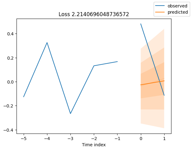