Autoregressive modelling with DeepAR and DeepVAR#
[1]:
import warnings

warnings.filterwarnings("ignore")
[2]:
import lightning.pytorch as pl
from lightning.pytorch.callbacks import EarlyStopping
import matplotlib.pyplot as plt
import pandas as pd
import torch

from pytorch_forecasting import Baseline, DeepAR, TimeSeriesDataSet
from pytorch_forecasting.data import NaNLabelEncoder
from pytorch_forecasting.data.examples import generate_ar_data
from pytorch_forecasting.metrics import MAE, SMAPE, MultivariateNormalDistributionLoss
Load data#
We generate a synthetic dataset to demonstrate the network’s capabilities. The data consists of a quadratic trend and a seasonality component.
[3]:
data = generate_ar_data(seasonality=10.0, timesteps=400, n_series=100, seed=42)
data["static"] = 2
data["date"] = pd.Timestamp("2020-01-01") + pd.to_timedelta(data.time_idx, "D")
data.head()
[3]:
| series | time_idx | value | static | date | |
|---|---|---|---|---|---|
| 0 | 0 | 0 | -0.000000 | 2 | 2020-01-01 |
| 1 | 0 | 1 | -0.046501 | 2 | 2020-01-02 |
| 2 | 0 | 2 | -0.097796 | 2 | 2020-01-03 |
| 3 | 0 | 3 | -0.144397 | 2 | 2020-01-04 |
| 4 | 0 | 4 | -0.177954 | 2 | 2020-01-05 |
[4]:
data = data.astype(dict(series=str))
[5]:
# create dataset and dataloaders
max_encoder_length = 60
max_prediction_length = 20

training_cutoff = data["time_idx"].max() - max_prediction_length

context_length = max_encoder_length
prediction_length = max_prediction_length

training = TimeSeriesDataSet(
    data[lambda x: x.time_idx <= training_cutoff],
    time_idx="time_idx",
    target="value",
    categorical_encoders={"series": NaNLabelEncoder().fit(data.series)},
    group_ids=["series"],
    static_categoricals=[
        "series"
    ],  # as we plan to forecast correlations, it is important to use series characteristics (e.g. a series identifier)
    time_varying_unknown_reals=["value"],
    max_encoder_length=context_length,
    max_prediction_length=prediction_length,
)

validation = TimeSeriesDataSet.from_dataset(
    training, data, min_prediction_idx=training_cutoff + 1
)
batch_size = 128
# synchronize samples in each batch over time - only necessary for DeepVAR, not for DeepAR
train_dataloader = training.to_dataloader(
    train=True, batch_size=batch_size, num_workers=0, batch_sampler="synchronized"
)
val_dataloader = validation.to_dataloader(
    train=False, batch_size=batch_size, num_workers=0, batch_sampler="synchronized"
)
Calculate baseline error#
Our baseline model predicts future values by repeating the last know value. The resulting SMAPE is disappointing and should be easy to beat.
[6]:
# calculate baseline absolute error
baseline_predictions = Baseline().predict(
    val_dataloader, trainer_kwargs=dict(accelerator="cpu"), return_y=True
)
SMAPE()(baseline_predictions.output, baseline_predictions.y)
GPU available: True (mps), used: False
TPU available: False, using: 0 TPU cores
IPU available: False, using: 0 IPUs
HPU available: False, using: 0 HPUs
[6]:
tensor(0.5462)
The DeepAR model can be easily changed to a DeepVAR model by changing the applied loss function to a multivariate one, e.g. MultivariateNormalDistributionLoss.
[7]:
pl.seed_everything(42)
import pytorch_forecasting as ptf

trainer = pl.Trainer(accelerator="cpu", gradient_clip_val=1e-1)
net = DeepAR.from_dataset(
    training,
    learning_rate=3e-2,
    hidden_size=30,
    rnn_layers=2,
    loss=MultivariateNormalDistributionLoss(rank=30),
    optimizer="Adam",
)
Global seed set to 42
GPU available: True (mps), used: False
TPU available: False, using: 0 TPU cores
IPU available: False, using: 0 IPUs
HPU available: False, using: 0 HPUs
Train network#
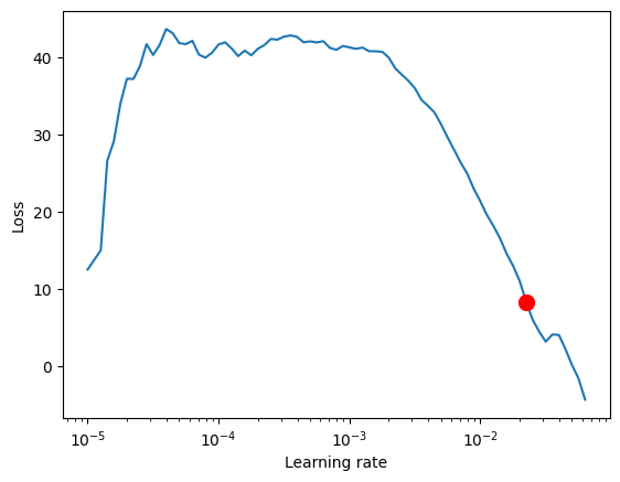
Finding the optimal learning rate using PyTorch Lightning is easy.
[ ]:
# find optimal learning rate
from pytorch_forecasting.tuning import Tuner

res = Tuner(trainer).lr_find(
    net,
    train_dataloaders=train_dataloader,
    val_dataloaders=val_dataloader,
    min_lr=1e-5,
    max_lr=1e0,
    early_stop_threshold=100,
)
print(f"suggested learning rate: {res.suggestion()}")
fig = res.plot(show=True, suggest=True)
net.hparams.learning_rate = res.suggestion()
LR finder stopped early after 76 steps due to diverging loss.
Learning rate set to 0.022387211385683406
Restoring states from the checkpoint path at /Users/JanBeitner/Documents/code/pytorch-forecasting/.lr_find_f89a547a-b375-400f-be1c-512fb11fc610.ckpt
Restored all states from the checkpoint at /Users/JanBeitner/Documents/code/pytorch-forecasting/.lr_find_f89a547a-b375-400f-be1c-512fb11fc610.ckpt
suggested learning rate: 0.022387211385683406
[9]:
early_stop_callback = EarlyStopping(
    monitor="val_loss", min_delta=1e-4, patience=10, verbose=False, mode="min"
)
trainer = pl.Trainer(
    max_epochs=30,
    accelerator="cpu",
    enable_model_summary=True,
    gradient_clip_val=0.1,
    callbacks=[early_stop_callback],
    limit_train_batches=50,
    enable_checkpointing=True,
)


net = DeepAR.from_dataset(
    training,
    learning_rate=1e-2,
    log_interval=10,
    log_val_interval=1,
    hidden_size=30,
    rnn_layers=2,
    optimizer="Adam",
    loss=MultivariateNormalDistributionLoss(rank=30),
)

trainer.fit(
    net,
    train_dataloaders=train_dataloader,
    val_dataloaders=val_dataloader,
)
GPU available: True (mps), used: False
TPU available: False, using: 0 TPU cores
IPU available: False, using: 0 IPUs
HPU available: False, using: 0 HPUs

  | Name                   | Type                               | Params
------------------------------------------------------------------------------
0 | loss                   | MultivariateNormalDistributionLoss | 0
1 | logging_metrics        | ModuleList                         | 0
2 | embeddings             | MultiEmbedding                     | 2.1 K
3 | rnn                    | LSTM                               | 13.9 K
4 | distribution_projector | Linear                             | 992
------------------------------------------------------------------------------
17.0 K    Trainable params
0         Non-trainable params
17.0 K    Total params
0.068     Total estimated model params size (MB)
`Trainer.fit` stopped: `max_epochs=30` reached.
[ ]:
best_model_path = trainer.checkpoint_callback.best_model_path
best_model = DeepAR.load_from_checkpoint(best_model_path)
[11]:
# best_model = net
predictions = best_model.predict(
    val_dataloader, trainer_kwargs=dict(accelerator="cpu"), return_y=True
)
MAE()(predictions.output, predictions.y)
GPU available: True (mps), used: False
TPU available: False, using: 0 TPU cores
IPU available: False, using: 0 IPUs
HPU available: False, using: 0 HPUs
[11]:
tensor(0.2782)
[12]:
raw_predictions = net.predict(
    val_dataloader,
    mode="raw",
    return_x=True,
    n_samples=100,
    trainer_kwargs=dict(accelerator="cpu"),
)
GPU available: True (mps), used: False
TPU available: False, using: 0 TPU cores
IPU available: False, using: 0 IPUs
HPU available: False, using: 0 HPUs
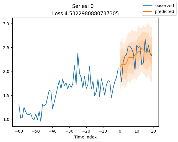
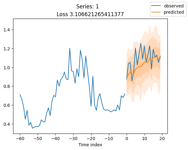
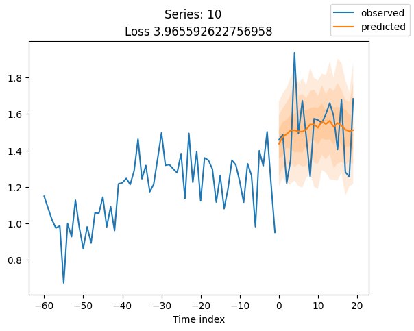
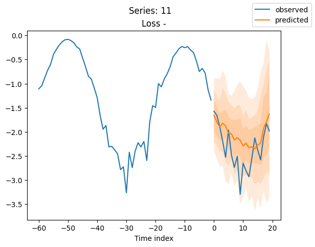
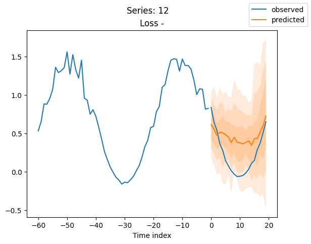
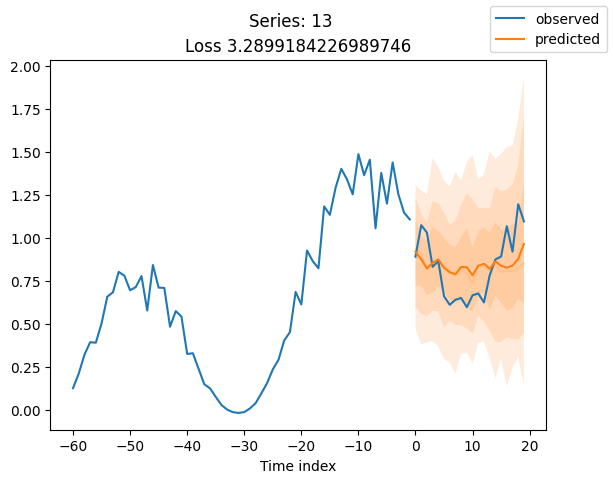
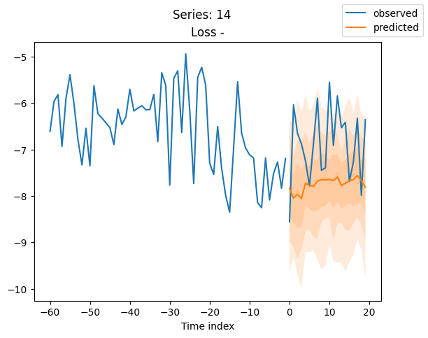
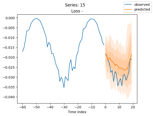
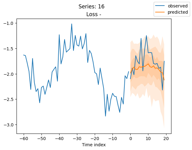
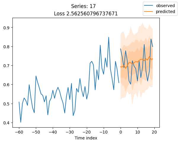
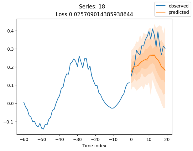
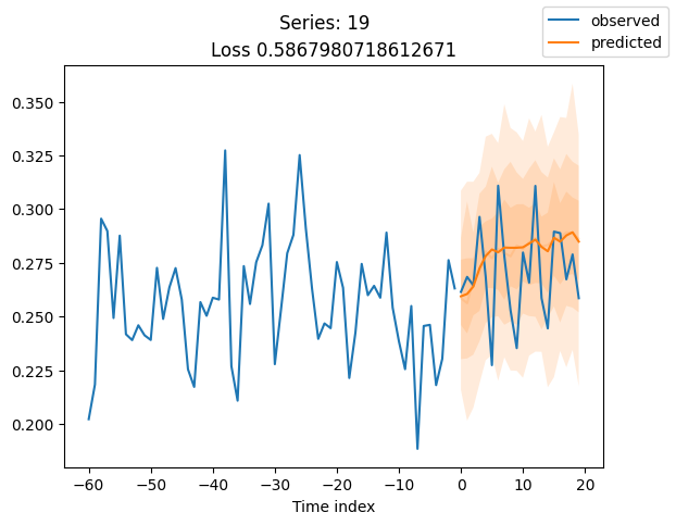
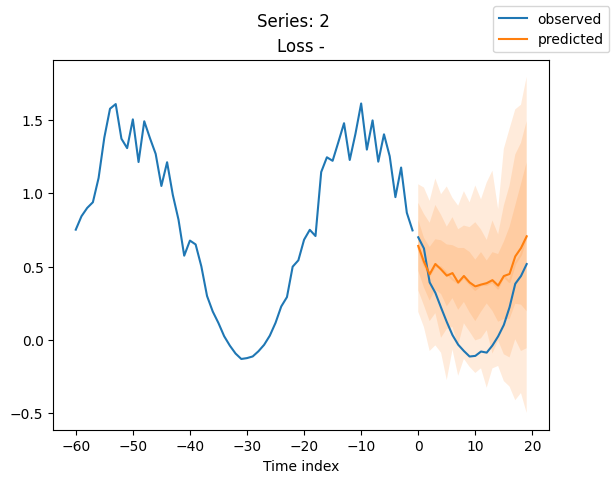
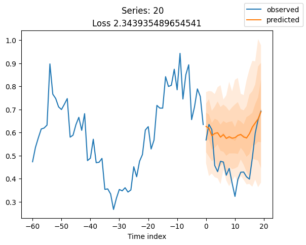
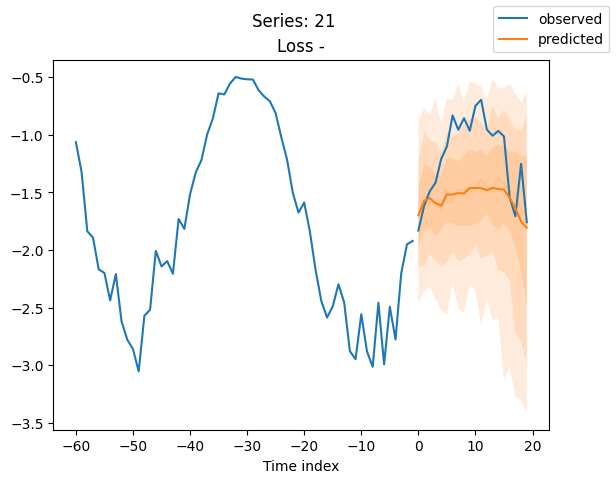
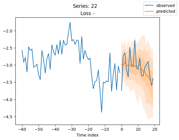
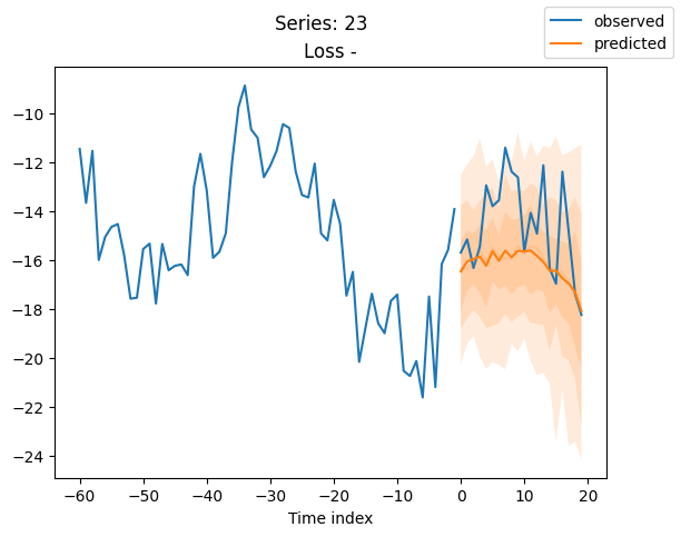
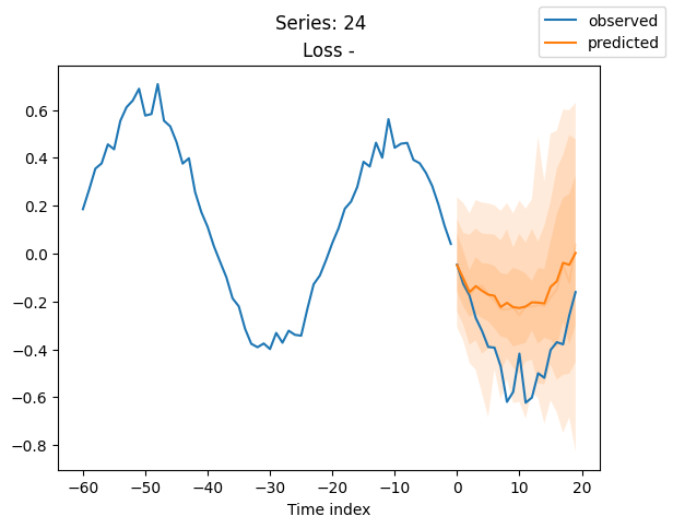
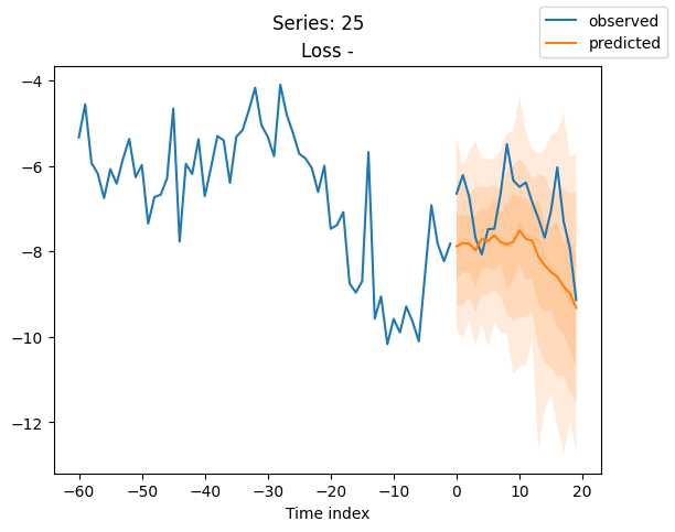
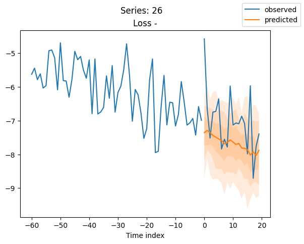
[13]:
series = validation.x_to_index(raw_predictions.x)["series"]
for idx in range(20):  # plot 10 examples
    best_model.plot_prediction(
        raw_predictions.x, raw_predictions.output, idx=idx, add_loss_to_title=True
    )
    plt.suptitle(f"Series: {series.iloc[idx]}")
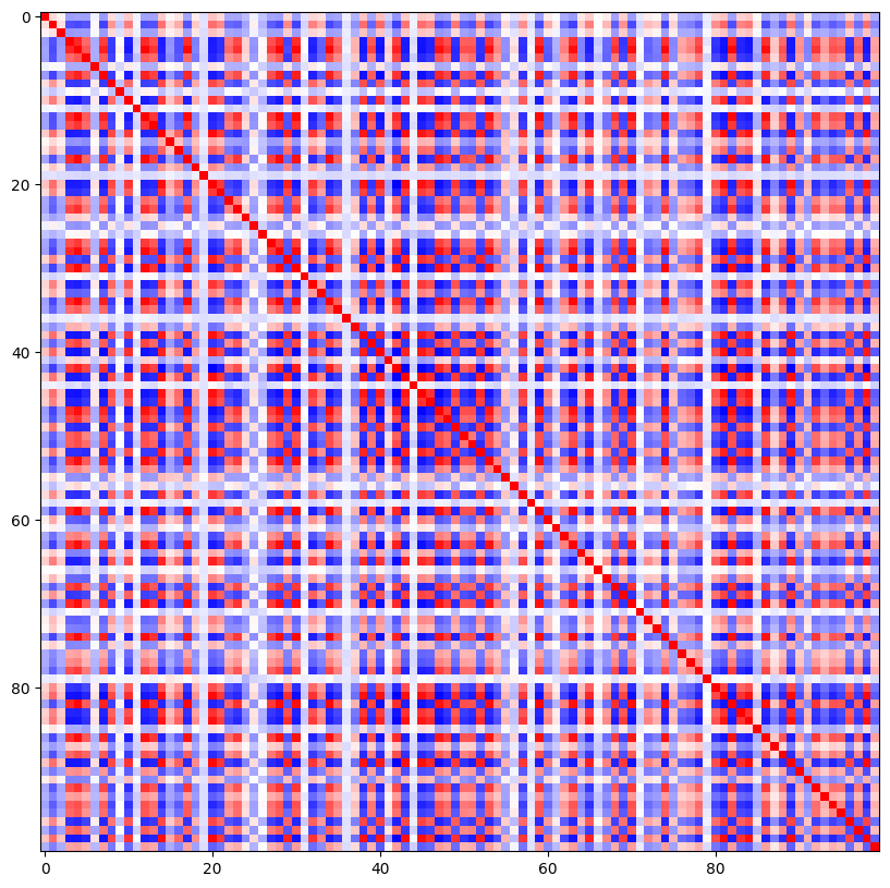
When using DeepVAR as a multivariate forecaster, we might be also interested in the correlation matrix. Here, there is no correlation between the series and we probably would need to train longer for this to show up.
[14]:
cov_matrix = best_model.loss.map_x_to_distribution(
    best_model.predict(
        val_dataloader,
        mode=("raw", "prediction"),
        n_samples=None,
        trainer_kwargs=dict(accelerator="cpu"),
    )
).base_dist.covariance_matrix.mean(0)

# normalize the covariance matrix diagonal to 1.0
correlation_matrix = cov_matrix / torch.sqrt(
    torch.diag(cov_matrix)[None] * torch.diag(cov_matrix)[None].T
)

fig, ax = plt.subplots(1, 1, figsize=(10, 10))
ax.imshow(correlation_matrix, cmap="bwr")
GPU available: True (mps), used: False
TPU available: False, using: 0 TPU cores
IPU available: False, using: 0 IPUs
HPU available: False, using: 0 HPUs
[14]:
<matplotlib.image.AxesImage at 0x2c4118d90>
[15]:
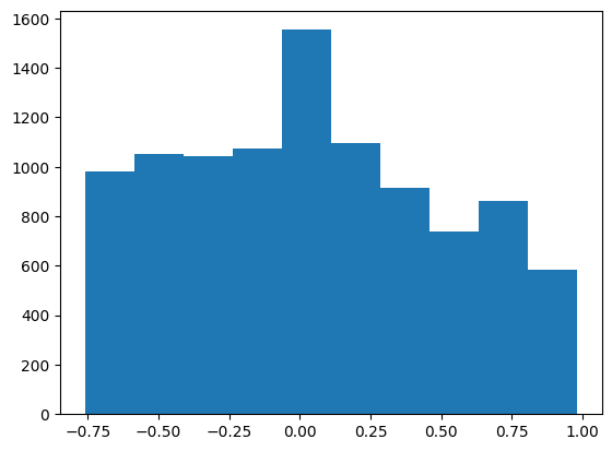
# distribution of off-diagonal correlations
plt.hist(correlation_matrix[correlation_matrix < 1].numpy())
[15]:
(array([ 982., 1052., 1042., 1072., 1554., 1098.,  916.,  738.,  862.,
         584.]),
 array([-0.76116514, -0.58684874, -0.4125323 , -0.23821589, -0.06389947,
         0.11041695,  0.28473336,  0.45904979,  0.63336623,  0.80768263,
         0.98199904]),
 <BarContainer object of 10 artists>)